ML-Kurs-SS2023/slides/03_ml_intro_mva.md

% Introduction to Data Analysis and Machine Learning in Physics: \ 3. Machine Learning Basics, Multivariate Analysis % Jörg Marks, Klaus Reygers % Studierendentage, 11-14 April 2023

Multi-variate analyses (MVA)

• General Question \vspace{0.1cm}

  There are 2 categories of distinguishable data, S and B, described by discrete variables. What are criteria for a separation of both samples?

  • Single criteria are not sufficient to distinguish S and B
  • Reduction of the variable space to probabilities for S or B \vspace{0.1cm}

• Classification of measurements using a set of observables $(V_1,V_2,....,V_n)$

  • find optimal separation conditions considering correlations

\begin{figure} \centering \includegraphics[width=0.8\textwidth]{figures/SandBcuts.jpeg} \end{figure}

Multi-variate analyses (MVA)

• Regression - in the multidimensional observable space $(V_1,V_2,....,V_n)$ a functional connection with optimal parameters is determined

\begin{figure} \centering \includegraphics[width=0.8\textwidth]{figures/regression.jpeg} \end{figure}

• supervised regression: model is known

• unsupervised regression: model is unknown

• for the parameter determination Maximum likelihood fits are used

MVA Classification in N Dimensions

For each event there are N measured variables

\begin{figure} \centering \includegraphics[width=0.9\textwidth]{figures/classificationVar.jpeg} \end{figure}

:::: columns :::: {.column width=70%}

• Search for a mathematical transformation F of the N dimensional input space to a one dimensional output space $F(\vec V) : \mathbb{R}^N \rightarrow \mathbb{R}$

• A simple cut in F implements a complex cut in the N dimensional variable space

• Determine $F(\vec V)$ using a model and fit the parameters
  :::: ::::{.column width=30%} \includegraphics[]{figures/response.jpeg} :::: :::

MVA Classification in N Dimensions

:::: columns :::: {.column width=60%}

• Parameters \newline Important measures to quantify quality \newline \newline Efficiency: $\epsilon = \frac{N_S (F>F_0)}{N_s}$ \newline Purity: $\pi = \frac{N_S (F>F_0)}{(N_s + N_B)(F>F_0)}$ :::: ::::{.column width=40%} \includegraphics[]{figures/response.jpeg} :::: ::: \vspace{0.3cm} :::: columns :::: {.column width=60%}
• Reciever Operations Characteristics (ROC) \newline Errors in classification \newline \includegraphics[width=0.7\textwidth]{figures/error.jpeg} :::: ::::{.column width=40%} \includegraphics[]{figures/roc.jpeg} :::: :::

MVA Classification in N Dimensions

:::: columns :::: {.column width=60%}

• Interpretation of $F(\vec V)$

  • The distributions of \textcolor{blue}{$F(\vec V|S)$} and \textcolor{red}{$F(\vec V|S)$} are interpreted as probability density functions (PDF), \textcolor{blue}{$PDF_S(F)$} and \textcolor{blue}{$PDF_B(F)$}

  • For a given $F_0$ the probability for signal and background for a given $S/B$ can be determined \newline $P ( data = S | F)= \frac {\color {blue} {f_S \cdot PDF_S(F)}} { \color {red} {f_B \cdot PDF_B(F)} + \color {blue} {f_S \cdot PDF_S(F)} }$ :::: ::::{.column width=40%} \includegraphics[]{figures/response.jpeg} :::: ::: \vspace{0.3cm}

• A cut in the one dimensional Variable $F(\vec V) =F_0$ and accepting all events on the right determines the signal and background efficiency (background rejection). A systematic change of $F(\vec V)$ gives the ROC curve. \newline

\definecolor{darkgreen}{RGB}{0,125,0}

• \color{darkgreen}{A cut in $F(\vec V)$ corresponds to a complex hyperplane, which can not neccessarily be described by a function.}

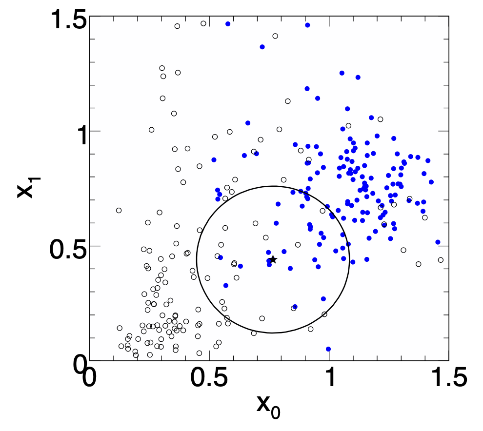
Simple Cuts in Variables

• The most simple classificator to select signal events are cuts in all variables which show a separation

  • The output is binary and not a probability on $S$ or $B$.

  • An optimization of the cuts is done by maximizing of the background suppression for given signal efficiencies.

  • Significance $sig = \epsilon_S \cdot N_S / \sqrt{ \epsilon_S \cdot N_S + \epsilon_B( \epsilon_S) N_B}$

\begin{figure} \centering \includegraphics[width=0.8\textwidth]{figures/cutInVariables.jpeg} \end{figure}

Fisher Discriminat

Idea: Find a plane, that the projection of the data on the plane gives an optimal separation of signal and background

:::: columns :::: {.column width=60%}

• The Fisher discriminat is the linear combination of all input variables \newline $F(\vec{V}) = \sum_i w_i \cdot V_i = \vec{w}^T \vec{V}$ \newline

• $\vec w$ defines the orientation of the plane. The coefficients are defined such that the difference of the expectation values of both classes is large and the variance is small. \newline $J( \vec{w} ) = \frac {( F_S - F_B )^2}{ \sigma_S^2 + \sigma_B^2 } = \frac { \vec{w}^T K \vec{w} }{ \vec{w}^T L \vec{w} }$ \newline with $K$ as covariance of the the expectation values $F_S -F_B$ and L is the sum

• For the separation a value $F_c$ is determined. :::: ::::{.column width=40%} \includegraphics[]{figures/fisher.jpeg} :::: :::

k-Nearest Neighbor Method (1)

$k$-NN classifier:

• Estimates probability density around the input vector
• $p(\vec x|S)$ and $p(\vec x|B)$ are approximated by the number of signal and background events in the training sample that lie in a small volume around the point $\vec x$

\vspace{2ex}

Algorithms finds $k$ nearest neighbors: $$ k = k_s + k_b $$

Probability for the event to be of signal type:

$$ p_s(\vec x) = \frac{k_s(\vec x)}{k_s(\vec x) + k_b(\vec x)} $$

k-Nearest Neighbor Method (2)

::: columns :::: {.column width=60%} Simplest choice for distance measure in feature space is the Euclidean distance: $$ R = |\vec x - \vec y|$$

Better: take correlations between variables into account:

$$ R = \sqrt{(\vec{x}-\vec{y})^T V^{-1} (\vec{x}-\vec{y})} $$ $$ V = \text{covariance matrix}, R = \text{"Mahalanobis distance"}$$

:::: :::: {.column width=40%} :::: :::

\vfill

The $k$-NN classifier has best performance when the boundary that separates signal and background events has irregular features that cannot be easily approximated by parametric learning methods.

Linear regression revisited

\vfill

::: columns :::: {.column width=50%} \small \textcolor{gray}{"Galton family heights data": \ origin of the term "regression"} \normalsize

:::: :::: {.column width=50%}

• data: ${x_i,y_i}$ \
• objective: predict $y = f(x)$
• model: $f(x; \vec \theta) = m x + b, \quad \vec \theta = (m, b)$
• loss function: $J(\theta|x,y) = \frac{1}{N} \sum_{i=1}^N (y_i - f(x_i))^2$
• model training: optimal parameters $\hat{\vec{\theta}} = \mathrm{arg,min} , J(\vec \theta)$

:::: :::

Linear regression

• Data: vectors with $p$ components ("features"): $\vec x = (x_1, ..., x_p)$

• $n$ observations: ${\vec x_i, y_i}, \quad i = 1, ..., n$

• Prediction for given vector $x$: $$ y = w_0 + w_1 x_1 + w_2 x_2 + ... + w_p x_p \equiv \vec w^\intercal \vec x \quad \text{where } x_0 := 1 $$

• Find weights that minimze loss function: $$\hat{\vec{w}} = \underset{\vec w}{\min} \sum_{i=1}^{n} (\vec w^\intercal \vec x_i - y_i)^2$$

• In case of linear regression closed-form solution exists: $$ \hat{\vec{w}} = (X^\intercal X)^{-1} X^\intercal \vec y \quad \text{where} ; X \in \mathbb{R}^{n \times p}$$

• $X$ is called the design matrix, row $i$ of $X$ is $\vec x_i$

Linear regression with regularization

::: columns :::: {.column width=45%}

• Standard loss function $$ C(\vec w) = \sum_{i=1}^{n} (\vec w^\intercal \vec x_i - y_i)^2 $$

• Ridge regression $$ C(\vec w) = \sum_{i=1}^{n} (\vec w^\intercal \vec x_i - y_i)^2 + \lambda |\vec w|^2$$

• LASSO regression $$ C(\vec w) = \sum_{i=1}^{n} (\vec w^\intercal \vec x_i - y_i)^2 + \lambda |\vec w| $$

:::: :::: {.column width=55%}

\vfill

\small \textcolor{gray}{LASSO regression tends to give sparse solutions (many components $w_j = 0$). This is why LASSO regression is also called sparse regression.} \normalsize :::: :::

Logistic regression (1)

• Consider binary classification task, e.g., $y_i \in {0,1}$
• Objective: Predict probability for outcome $y=1$ given an observation $\vec x$
• Starting with linear "score" $$ s = w_0 + w_1 x_1 + w_2 x_2 + ... + w_p x_p \equiv \vec w^\intercal \vec x$$
• Define function that translates $s$ into a quantity that has the properties of a probability $$ \sigma(s) = \frac{1}{1+e^{-s}} $$
• We would like to determine the optimal weights for a given training data set. They result from the maximum-likelihood principle.

Logistic regression (2)

• Consider feature vector $\vec x$. For a given set of weights $\vec w$ the model predicts
  • a probability $p(1|\vec w) = \sigma(\vec w^\intercal \vec x)$ for outcome $y=1$
  • a probabiltiy $p(0|\vec w) = 1 - \sigma(\vec w^\intercal \vec x)$ for outcome $y=0$
• The probability $p(y_i | \vec w)$ defines the likelihood $L_i(\vec w) = p(y_i | \vec w)$ (the likelihood is a function of the parameters $\vec w$ and the observations $y_i$ are fixed).
• Likelihood for the full data sample ($n$ observations) $$ L(\vec w) = \prod_{i=1}^n L_i(\vec w) = \prod_{i=1}^n \sigma(\vec w^\intercal \vec x)^{y_i} ,(1-\sigma(\vec w^\intercal \vec x))^{1-y_i} $$
• Maximizing the log-likelihood $\ln L(\vec w)$ corresponds to minimizing the loss function $$ C(\vec w) = - \ln L(\vec w) = \sum_{i=1}^n - y_i \ln \sigma(\vec w^\intercal \vec x) - (1-y_i) \ln(1-\sigma(\vec w^\intercal \vec x))$$
• This is nothing else but the cross-entropy loss function

Example 1 - Probability of passing an exam (logistic regression) (1)

Objective: predict the probability that someone passes an exam based on the number of hours studying

$$ p_\mathrm{pass} = \sigma(s) = \frac{1}{1+e^{-s}}, \quad s = w_1 t + w_0, \quad t = \text{# hours}$$

::: columns :::: {.column width=40%}

• Data set: \
  • preparation $t$ time in hours
  • passed / not passes (0/1)
• Parameters need to be determined through numerical minimization
  • $w_0 = -4.0777$
  • $w_1 = 1.5046$

\vspace{1.5ex} \footnotesize \textcolor{gray}{03_ml_basics_logistic_regression.ipynb} \normalsize :::: :::: {.column width=60%} {width=90%} :::: :::

Example 1 - Probability of passing an exam (logistic regression) (2)

\footnotesize \textcolor{gray}{Read data from file:}

# data: 1. hours studies, 2. passed (0/1)  
df = pd.read_csv(filename, engine='python', sep='\s+')
x_tmp = df['hours_studied'].values
x = np.reshape(x_tmp, (-1, 1))
y = df['passed'].values

\vfill \textcolor{gray}{Fit the data:}

from sklearn.linear_model import LogisticRegression
clf = LogisticRegression(penalty='none', fit_intercept=True)
clf.fit(x, y);

\vfill \textcolor{gray}{Calculate predictions:}

hours_studied_tmp = np.linspace(0., 6., 1000)
hours_studied = np.reshape(hours_studied_tmp, (-1, 1))
y_pred = clf.predict_proba(hours_studied)

\normalsize

Precision and recall

::: columns :::: {.column width=50%} \textcolor{blue}{Precision:}
Fraction of correctly classified instances among all instances that obtain a certain class label.

$$ \text{precision} = \frac{\text{TP}}{\text{TP} + \text{FP}} $$

\begin{center} \textcolor{gray}{"purity"} \end{center}

:::: :::: {.column width=50%} \textcolor{blue}{Recall:}
Fraction of positive instances that are correctly classified. \vspace{2.9ex}

$$ \text{recall} = \frac{\text{TP}}{\text{TP} + \text{FN}} $$

\begin{center} \textcolor{gray}{"efficiency"} \end{center}

:::: ::: \vfill \begin{center} \textcolor{gray}{TP: true positives, FP: false positives, FN: false negatives} \end{center}

Example 2: Heart disease data set (logistic regression) (1)

\scriptsize \textcolor{gray}{Read data:}

filename = "https://www.physi.uni-heidelberg.de/~reygers/lectures/2023/ml/data/heart.csv"
df = pd.read_csv(filename)
df

\vfill 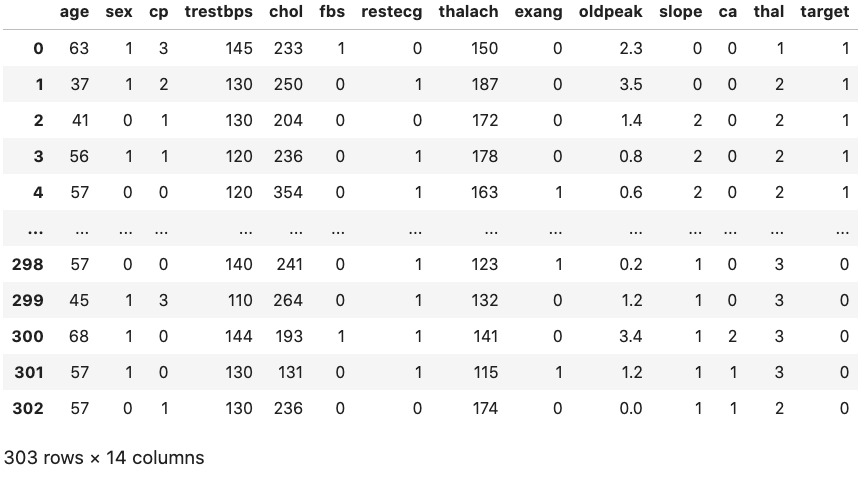{width=70%} \normalsize \vspace{1.5ex} \footnotesize \textcolor{gray}{03_ml_basics_log_regr_heart_disease.ipynb} \normalsize

Example 2: Heart disease data set (logistic regression) (2)

\footnotesize

\textcolor{gray}{Define array of labels and feature vectors}

y = df['target'].values
X = df[[col for col in df.columns if col!="target"]]

\vfill \textcolor{gray}{Generate training and test data sets}

from sklearn.model_selection import train_test_split
X_train, X_test, y_train, y_test = train_test_split(X, y, test_size=0.5, shuffle=True)

\vfill \textcolor{gray}{Fit the model}

from sklearn.linear_model import LogisticRegression
lr = LogisticRegression(penalty='none', fit_intercept=True, max_iter=1000, tol=1E-5)
lr.fit(X_train, y_train)

\normalsize

Example 2: Heart disease data set (logistic regression) (3)

\footnotesize \textcolor{gray}{Test predictions on test data set:}

from sklearn.metrics import classification_report
y_pred_lr = lr.predict(X_test)
print(classification_report(y_test, y_pred_lr))

\vfill \textcolor{gray}{Output:}

              precision    recall  f1-score   support

           0       0.75      0.86      0.80        63
           1       0.89      0.80      0.84        89

    accuracy                           0.82       152
   macro avg       0.82      0.83      0.82       152
weighted avg       0.83      0.82      0.82       152

Example 2: Heart disease data set (logistic regression) (4)

\textcolor{gray}{Compare to another classifier usinf the \textit{receiver operating characteristic} (ROC) curve} \vfill \textcolor{gray}{Let's take the random forest classifier} \footnotesize

from sklearn.ensemble import RandomForestClassifier
rf = RandomForestClassifier(max_depth=3)
rf.fit(X_train, y_train)

\normalsize \vfill \textcolor{gray}{Use \texttt{roc_curve} from scikit-learn} \footnotesize

from sklearn.metrics import roc_curve

y_pred_prob_lr = lr.predict_proba(X_test) # predicted probabilities
fpr_lr, tpr_lr, _ = roc_curve(y_test, y_pred_prob_lr[:,1])

y_pred_prob_rf = rf.predict_proba(X_test) # predicted probabilities
fpr_rf, tpr_rf, _ = roc_curve(y_test, y_pred_prob_rf[:,1])

\normalsize

Example 2: Heart disease data set (logistic regression) (5)

::: columns :::: {.column width=50%} \scriptsize

plt.plot(tpr_lr, 1-fpr_lr, label="log. regression")
plt.plot(tpr_rf, 1-fpr_rf, label="random forest")

\vspace{5ex}

\normalsize \textcolor{gray}{Classifiers can be compared with the \textit{area under curve} (AUC) score.} \scriptsize

from sklearn.metrics import roc_auc_score
auc_lr = roc_auc_score(y_test,y_pred_lr)
auc_rf = roc_auc_score(y_test,y_pred_rf)
print(f"AUC scores: {auc_lr:.2f}, {auc_knn:.2f}")

\vspace{5ex} \normalsize \textcolor{gray}{This gives} \scriptsize

AUC scores: 0.82, 0.83

\normalsize

:::: :::: {.column width=50%} \begin{figure} \centering \includegraphics[width=0.96\textwidth]{figures/03_ml_basics_log_regr_heart_disease.pdf} \end{figure} :::: :::

Multinomial logistic regression: Softmax function

In the previous example we considered two classes (0, 1). For multi-class classification, the logistic function can generalized to the softmax function. \vfill Now consider $k$ classes and let $s_i$ be the score for class $i$: $\vec s = (s_1, ..., s_k)$ \vfill A probability for class $i$ can be predicted with the softmax function: $$ \sigma(\vec s)i = \frac{e^{s_i}}{\sum{j=1}^k e^{s_j}} \quad \text{ for } \quad i = 1, ... , k $$ The softmax functions is often used as the last activation function of a neural network in order to predict probabilities in a classification task. \vfill Multinomial logistic regression is also known as softmax regression.

Example 3: Iris data set (softmax regression) (1)

Iris flower data set

• Introduced 1936 in a paper by Ronald Fisher
• Task: classify flowers
• Three species: iris setosa, iris virginica and iris versicolor
• Four features: petal width and length, sepal width/length, in centimeters

::: columns :::: {.column width=40%} \begin{figure} \centering \includegraphics[width=0.95\textwidth]{figures/iris_dataset.png} \end{figure} :::: :::: {.column width=60%}

\vspace{2ex}

\footnotesize \textcolor{gray}{03_ml_basics_iris_softmax_regression.ipynb}

\vspace{19ex}

\scriptsize https://archive.ics.uci.edu/ml/datasets/Iris

https://en.wikipedia.org/wiki/Iris_flower_data_set \normalsize :::: :::

Example 3: Iris data set (softmax regression) (2)

\textcolor{gray}{Get data set} \footnotesize

# import some data to play with
# columns: Sepal Length, Sepal Width, Petal Length and Petal Width
iris = datasets.load_iris()
X = iris.data
y = iris.target

# split data into training and test data sets
x_train, x_test, y_train, y_test = train_test_split(X, y, test_size=0.5, random_state=42)

\normalsize \vfill

\textcolor{gray}{Softmax regression} \footnotesize

from sklearn.linear_model import LogisticRegression
log_reg = LogisticRegression(multi_class='multinomial', penalty='none')
log_reg.fit(x_train, y_train);

\normalsize

Example 3 : Iris data set (softmax regression) (3)

::: columns :::: {.column width=70%} \textcolor{gray}{Accuracy and confusion matrix for different classifiers} \footnotesize

for clf in [log_reg, kn_neigh, fisher_ld]:
    y_pred = clf.predict(x_test)
    acc = accuracy_score(y_test, y_pred)
    print(type(clf).__name__)
    print(f"accuracy: {acc:0.2f}")

    # confusion matrix: 
    # columns: true class, row: predicted class
    print(confusion_matrix(y_test, y_pred),"\n")

\normalsize :::: :::: {.column width=30%}

\footnotesize

LogisticRegression
accuracy: 0.96
[[29  0  0]
 [ 0 23  0]
 [ 0  3 20]] 

KNeighborsClassifier
accuracy: 0.95
[[29  0  0]
 [ 0 23  0]
 [ 0  4 19]] 

LinearDiscriminantAnalysis
accuracy: 0.99
[[29  0  0]
 [ 0 23  0]
 [ 0  1 22]] 

\normalsize :::: :::

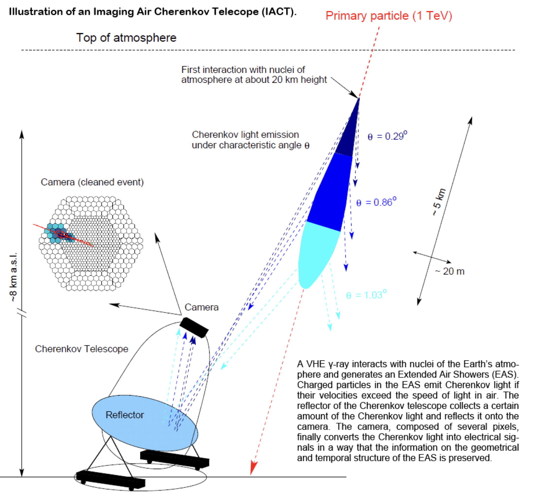
Exercise 1: Classification of air showers measured with the MAGIC telescope

::: columns :::: {.column width=50%}

\small

• Cosmic gamma rays (30 GeV - 30 TeV).
• Cherenkov light from air showers
• Background: air showers caused by hadrons. \normalsize

\begin{figure} \centering \includegraphics[width=0.85\textwidth]{figures/magic_photo_small.png} \end{figure} :::: :::: {.column width=50%} :::: :::

Exercise 1: Classification of air showers measured with the MAGIC telescope

\begin{figure} \centering \includegraphics[width=0.75\textwidth]{figures/magic_shower_em_had_small.png} \end{figure} ::: columns :::: {.column width=50%} \begin{center} Gamma shower \end{center} :::: :::: {.column width=50%} \begin{center} Hadronic shower \end{center} :::: :::

Exercise 1: Classification of air showers measured with the MAGIC telescope

\begin{figure} \centering \includegraphics[width=0.95\textwidth]{figures/magic_shower_parameters.png} \end{figure}

Exercise 1: Classification of air showers measured with the MAGIC telescope

MAGIC data set
\tiny \textcolor{gray}{https://archive.ics.uci.edu/ml/datasets/magic+gamma+telescope} \normalsize

\scriptsize

1.  fLength:  continuous  # major axis of ellipse [mm]
2.  fWidth:   continuous  # minor axis of ellipse [mm] 
3.  fSize:    continuous  # 10-log of sum of content of all pixels [in #phot]
4.  fConc:    continuous  # ratio of sum of two highest pixels over fSize  [ratio]
5.  fConc1:   continuous  # ratio of highest pixel over fSize  [ratio]
6.  fAsym:    continuous  # distance from highest pixel to center, projected onto major axis [mm]
7.  fM3Long:  continuous  # 3rd root of third moment along major axis  [mm] 
8.  fM3Trans: continuous  # 3rd root of third moment along minor axis  [mm]
9.  fAlpha:   continuous  # angle of major axis with vector to origin [deg]
10. fDist:    continuous  # distance from origin to center of ellipse [mm]
11. class:    g,h         # gamma (signal), hadron (background)

g = gamma (signal):     12332
h = hadron (background): 6688

For technical reasons, the number of h events is underestimated.
In the real data, the h class represents the majority of the events.

\normalsize

Exercise 1: Classification of air showers measured with the MAGIC telescope

\small \textcolor{gray}{03_ml_basics_ex_1_magic.ipynb} \normalsize

a) Create for each variable a figure with a plot for gammas and hadrons overlayed. b) Create training and test data set. The test data should amount to 50% of the total data set. c) Define the logistic regressor and fit the training data d) Determine the model accuracy and the AUC score e) Plot the ROC curve (background rejection vs signal efficiency)

General remarks on multi-variate analyses (MVAs)

• MVA Methods
  • More effective than classic cut-based analyses
  • Take correlations of input variables into account \vfill
• Important: find good input variables for MVA methods
  • Good separation power between S and B
  • No strong correlation among variables
  • No correlation with the parameters you try to measure in your signal sample! \vfill
• Pre-processing
  • Apply obvious variable transformations and let MVA method do the rest
  • Make use of obvious symmetries: if e.g. a particle production process is symmetric in polar angle $\theta$ use $|\cos \theta|$ and not $\cos \theta$ as input variable
  • It is generally useful to bring all input variables to a similar numerical range

Example of feature transformation

\begin{figure} \centering \includegraphics[width=0.95\textwidth]{figures/feature_transformation.png} \end{figure}

Exercise 2: Data preprocessing

a) Read the description of the sklearn.preprocessing package.

b) Start from the example notebook on the logistic regression for the heart disease data set (03_ml_basics_log_regr_heart_disease.ipynb). Pre-process the heart disease data set according to the given example. Does preprocessing make a difference in this case?