26 KiB
| title | author | date |
|---|---|---|
| | Introduction to Data Analysis and Machine Learning in Physics: | 5. Neural networks | Martino Borsato, Jörg Marks, Klaus Reygers | Studierendentage, 11-14 April 2022 |
Exercises
- Exercise 1: Learn XOR with a MLP
- Exercise 2: Visualising decision boundaries of classifiers
- Exercise 3: Boston house prices (MLP regression)
- Exercise 4: Training a digit-classification neural network on the MNIST dataset using Keras
Perceptron (1)
::: columns :::: {.column width=65%} \begin{center} \includegraphics[width=0.40\textwidth]{figures/perceptron_weighted_sum.png} \vspace{1ex} \includegraphics[width=0.75\textwidth]{figures/perceptron_retina.png} \end{center} :::: :::: {.column width=35%}
h(\vec x) = \begin{cases}1 & \text{if }\ \vec w \cdot \vec x + b > 0,\\0 & \text{otherwise}\end{cases}\begin{center} \includegraphics[width=0.95\textwidth]{figures/perceptron_photo.png} \tiny \textcolor{gray}{Mark 1 Perceptron. Frank Rosenblatt (1961)} \normalsize \end{center} :::: ::: \footnotesize \vspace{2ex} \textcolor{gray}{The perceptron was designed for image recognition. It was first implemented in hardware (400 photocells, weights = potentiometer settings).} \normalsize
Perceptron (2)
::: columns :::: {.column width=60%}
- McCulloch–Pitts (MCP) neuron (1943)
- First mathematical model of a biological neuron
- Boolean input
- Equal weights for all inputs
- Threshold hardcoded
- Improvements by Rosenblatt
- Different weights for inputs
- Algorithm to update weights and threshold given labeled training data
\vfill
Shortcoming of the perceptron: \newline it cannot learn the XOR function \newline \tiny \textcolor{gray}{Minsky, Papert, 1969} \normalsize
::::
:::: {.column width=40%}
 {width=80%}
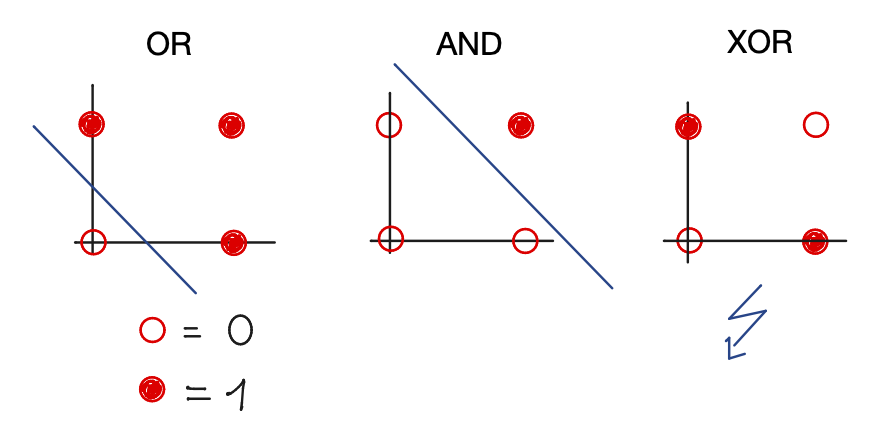 \small \textcolor{gray}{XOR: not linearly separable } \normalsize
:::: :::
The biological inspiration: the neuron
\begin{figure} \centering \includegraphics[width=0.95\textwidth]{figures/neuron.png} \end{figure}
Non-linear transfer / activation function
Discriminant: y(\vec x) = h\left( w_0 + \sum_{i=1}^n w_i x_i \right)
Examples for function h: \newline
\frac{1}{1+e^{-x}} \; \text{("sigmoid" or "logistic" function)}, \quad \tanh x ::: columns :::: {.column width=50%} \begin{figure} \centering \includegraphics[width=0.75\textwidth]{figures/logistic_fct.png} \end{figure} :::: :::: {.column width=50%} \vspace{3ex} Non-linear activation function needed in neural networks when feature space is not linearly separable. \newline
\small \textcolor{gray}{Neural net with linear activation functions is just a perceptron} \normalsize :::: :::
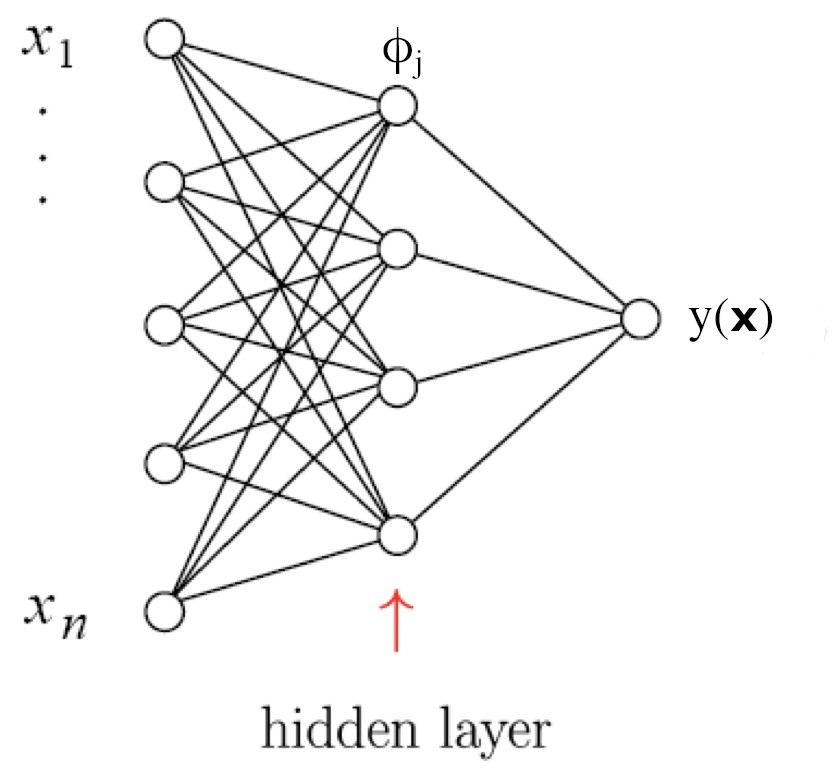
Feedforward neural network with one hidden layer
::: columns
:::: {.column width=60%}
 {width=80%}
::::
:::: {.column width=40%}
{width=80%}
::::
:::: {.column width=40%}
\phi_i(\vec x) = h\left(w_{i0}^{(1)} + \sum_{j=1}^n w_{ij}^{(1)} x_j\right) \vfill
y(\vec x) = h\left( w_{10}^{(2)} + \sum_{j=1}^m w_{1j}^{(2)} \phi_j(\vec x)\right) \vfill
\vspace{2ex}
\footnotesize
\textcolor{gray}{superscripts indicates layer number, i.e., w_{ij}^{(1)} refers to the input weights of neuron i in the hidden layer (= layer 1).}
\normalsize
:::: ::: \begin{center} Straightforward to generalize to multiple hidden layers \end{center}
Neural network output and decision boundaries
::: columns :::: {.column width=75%} \begin{figure} \centering \includegraphics[width=\textwidth]{figures/nn_decision_boundary.png} \end{figure} :::: :::: {.column width=25%} \vspace{3ex} \footnotesize \textcolor{gray}{P. Bhat, Multivariate Analysis Methods in Particle Physics, inspirehep.net/record/879273} \normalsize :::: :::
Fun with neural nets in the browser
\begin{figure} \centering \includegraphics[width=\textwidth]{figures/tf_playground.png} \end{figure} \tiny \textcolor{gray}{http://playground.tensorflow.org} \normalsize
Backpropagation (1)
Start with an initial guess \vec w_0 for the weights an then update weights after each training event:
\vec w^{(\tau+1)} = \vec w^{(\tau)} - \eta \nabla E_a(\vec w^{(\tau)}), \quad \eta = \text{learning rate}Gradient descent: \begin{figure} \centering \includegraphics[width=0.46\textwidth]{figures/gradient_descent.png} \end{figure}
Backpropagation (2)
::: columns
:::: {.column width=40%}
\vspace{6ex}
{width=100%}
::::
:::: {.column width=60%}
Let's write network output as follows:
\begin{align*}
y(\vec x) &= h(u(\vec x)); \quad u(\vec x) = \sum_{j=0}^m w_{1j}^{(2)} \phi_j(\vec x) \
\phi_j(\vec x) &= h\left( \sum_{k=0}^n w_{jk}^{(1)} x_k\right)
\equiv h\left( v_j(\vec x) \right)
\end{align*}
For E_a = \frac{1}{2} (y_a - t_a)^2 one obtains for the weights from hidden layer to output:
\begin{align*}
\frac{\partial E_a}{\partial w_{1j}^{(2)}} &= (y_a -t_a) h'(u(\vec x_a)) \frac{\partial u}{\partial w_{1j}^{(2)}} \
&= (y_a -t_a) h'(u(\vec x_a)) \phi_j(\vec x_a)
\end{align*}
::::
:::
\vspace{2ex}
Further application of the chain rule gives weights from input to hidden layer.
Backpropagation (3)
Backpropagation summary
- Make prediction for a given training instance (forward pass)
- Calculate error (value of loss function)
- Go backwards and determine the contribution of each weight (reverse pass)
- Adjust the weights to reduce the error
\vfill
Practical considerations:
- Nowadays, people will implements neural networks with frameworks like Keras or TensorFlow
- No need to implement backpropagation yourself
- TensorFlow efficiently calculates gradient function based on a kind of symbolic differentiation
More on gradient descent
::: columns :::: {.column width=60%}
- Stochastic gradient descent
- just uses one training event at a time
- fast, but quite irregular approach to the minimum
- can help escape local minima
- one can decrease learning rate to settle at the minimum ("simulated annealing")
- Batch gradient descent
- use entire training sample to calculate gradient of loss function
- computationally expensive
- Mini-batch gradient descent
- calculate gradient for a random sub-sample of the training set
:::: :::: {.column width=40%} \begin{figure} \centering \includegraphics[width=0.7\textwidth]{figures/stochastic_gradient_descent.png} \end{figure} \begin{figure} \centering \includegraphics[width=\textwidth]{figures/gradient_descent_cmp.png} \end{figure} :::: :::
Universal approximation theorem
::: columns
:::: {.column width=60%}
"A feed-forward network with a single hidden layer containing a finite number of neurons (i.e., a multilayer perceptron), can approximate continuous functions on compact subsets of \mathbb{R}^n."
\vspace{5ex}
One of the first versions of the theorem was proved by George Cybenko in 1989 for sigmoid activation functions
\vspace{5ex}
The theorem does not touch upon the algorithmic learnability of those parameters
:::: :::: {.column width=40%} \begin{figure} \centering \includegraphics[width=\textwidth]{figures/ann.png} \end{figure} :::: :::
Deep neural networks
Deep networks: many hidden layers with large number of neurons
::: columns :::: {.column width=45%}
- Challenges
- Hard too train ("vanishing gradient problem")
- Training slow
- Risk of overtraining :::: :::: {.column width=55%}
- Big progress in recent years
- Interest in NN waned before ca. 2006
- Milestone: paper by G. Hinton (2006): "learning for deep belief nets"
- Image recognition, AlphaGo, …
- Soon: self-driving cars, … :::: ::: \begin{figure} \centering \includegraphics[width=0.5\textwidth]{figures/dnn.png} \end{figure}
Drawbacks of the sigmoid activation function
::: columns :::: {.column width=50%} \includegraphics[width=.75\textwidth]{figures/sigmoid.png} :::: :::: {.column width=50%}
\sigma(x) = \frac{1}{1 + e^{-x}} \vspace{3ex}
- Saturated neurons “kill” the gradients
- Sigmoid outputs are not zero-centered
- exp() is a bit compute expensive :::: :::
Activation functions
\begin{figure} \centering \includegraphics[width=\textwidth]{figures/activation_functions.png} \end{figure}
ReLU
::: columns :::: {.column width=50%} \includegraphics[width=.75\textwidth]{figures/relu.png} :::: :::: {.column width=50%}
f(x) = \max(0,x) \vspace{1ex}
- Does not saturate (in +region)
- Very computationally efficient
- Converges much faster than sigmoid tanh in practice
- Actually more biologically plausible than sigmoid
- But: gradient vanishes for
x < 0
:::: :::
Bias-variance tradeoff (1)
Goal: generalization of training data
- Simple models (few parameters): danger of bias
- \textcolor{gray}{Classifiers with a small number of degrees of freedom are less prone to statistical fluctuations: different training samples would result in similar classification boundaries ("small variance")}
- Complex models (many parameters): danger of overfitting
- \textcolor{gray}{large variance of decision boundaries for different training samples}
Bias-variance tradeoff (2)
\begin{figure} \centering \includegraphics[trim=4cm 0cm 4cm 0cm, width=\textwidth]{figures/underfitting_overfitting.pdf} \end{figure}
Example of overtraining
Too many neurons/layers make a neural network too flexible \newline \to overtraining
\begin{figure} \centering \includegraphics[width=0.9\textwidth]{figures/example_overtraining.png} \end{figure}
Monitoring overtraining
Monitor fraction of misclassified events (or loss function:) \begin{figure} \centering \includegraphics[width=0.8\textwidth]{figures/monitoring_overtraining.png} \end{figure}
Regularization: Avoid overfitting
\scriptsize
\hfill \textcolor{gray}{http://cs231n.stanford.edu/slides}
\normalsize
\begin{figure}
\centering
\includegraphics[width=0.75\textwidth]{figures/regularization.png}
\end{figure}
\begin{center}
L_1 regularization: R(W) = \sum_k |W_k|, L_2 regularization: $R(W) = \sum_k W_k^2$
\end{center}
Another approach to prevent overfitting: Dropout
- Randomly remove nodes during training
- Avoid co-adaptation of nodes \begin{figure} \centering \includegraphics[width=0.8\textwidth]{figures/dropout.png} \end{figure} \scriptsize \textcolor{gray}{Srivastava et al.,} \textcolor{gray}{"Dropout: A Simple Way to Prevent Neural Networks from Overfitting"} \normalsize
Pros and cons of multi-layer perceptrons
\textcolor{green}{Pros}
- Capability to learn non-linear models
\vspace{3ex}
\textcolor{red}{Cons}
- Loss function can have several local minima
- Hyperparameters need to be tuned
- \textcolor{gray}{number of layers, neurons per layer, and training iterations}
- Sensitive to feature scaling
- \textcolor{gray}{preprocessing needed (e.g., scaling of all feature to range [0,1])}
Example 1: Boston house prices (MLP regression) (1)
- Objective: predict house prices in Boston suburbs in the mid-1970s
- Boston house data set: 506 instances, 13 features
\footnotesize
    - CRIM     per capita crime rate by town
    - ZN       proportion of residential land zoned for lots over 25,000 sq.ft.
    - INDUS    proportion of non-retail business acres per town
    - CHAS     Charles River dummy variable (= 1 if tract bounds river; 0 otherwise)
    - NOX      nitric oxides concentration (parts per 10 million)
    - RM       average number of rooms per dwelling
    - AGE      proportion of owner-occupied units built prior to 1940
    - DIS      weighted distances to five Boston employment centres
    - RAD      index of accessibility to radial highways
    - TAX      full-value property-tax rate per $10,000
    - PTRATIO  pupil-teacher ratio by town
    - B        1000(Bk - 0.63)^2 where Bk is the proportion of blacks by town
    - LSTAT    % lower status of the population
    - MEDV     Median value of owner-occupied homes in $1000's
\footnotesize \textcolor{gray}{05_neural_networks_boston_house_prices.ipynb}
Example 1: Boston house prices (MLP regression) (2)
boston = datasets.load_boston()
X = boston.data
y = boston.target

from sklearn.neural_network import MLPRegressor
mlp = MLPRegressor(hidden_layer_sizes=(100),
	activation='logistic', random_state=1, max_iter=5000)
mlp.fit(X_train, y_train)

y_pred_mlp = mlp.predict(X_test)

rms = np.sqrt(mean_squared_error(y_test, y_pred_mlp))
print(f"root mean square error {rms:.2f}")
Example 1: Boston house prices (MLP regression) (3)
\begin{center} \includegraphics[width=0.7\textwidth]{figures/boston_house_prices.pdf} \end{center}
Exercise 1: XOR
\small \textcolor{gray}{05_neural_networks_ex_1_xor.ipynb} \normalsize
::: columns :::: {.column width=60%} a) Define a multi-layer perceptron classifier that learns the XOR problem. \scriptsize
	from sklearn.neural_network import MLPClassifier

	X = [[0, 0], [0, 1], [1, 0], [1, 1]]
	y = [0, 1, 1, 0]
\normalsize b) Define a multi-layer perceptron regressor that fits the depicted 2d data (see notebook).
c) Plot the mean square error vs. the number of number of training epochs for b).
::::
:::: {.column width=40%}
\vspace{10ex}

Exercise 2: Visualising decision boundaries of classifiers
\small \textcolor{gray}{05_neural_networks_ex_2_decision_boundaries.ipynb} \normalsize
\vspace{5ex}
Visualize the decision boundaries of a scikit-learn decision tree, a scikit-learn multi-layer perceptron, and XGBoost for different toy data sets.
Exercise 3: Boston house prices (hyperparameter optimization)
\small \textcolor{gray}{05_neural_networks_ex_3_boston_house_prices.ipynb} \normalsize
\vspace{5ex}
a) Can you find better hyperparameters (number of hidden layers, neurons per layer, loss function, ...)? Try this first by hand. b) Now use \textcolor{gray}{sklearn.model_selection.GridSearchCV} to find optimal parameters.
TensorFlow
::: columns :::: {.column width=70%}
- Powerful open source library with a focus on deep neural networks
- Performs computations of data flow graphs
- Takes care of computing gradients of the defined functions (\textit{automatic differentiation})
- Computations in parallel on multiple CPUs or GPUs
- Developed by the Google Brain team
- Initial release in 2015
- https://www.tensorflow.org/
:::: :::: {.column width=30%} \begin{center} \includegraphics[width=0.7\textwidth]{figures/tensorflow.png} \end{center} :::: :::
Keras
::: columns :::: {.column width=70%}
- Open-source library providing high-level building blocks for developing deep-learning models
- Uses TensorFlow as \textit{backend engine} for low-level tensor manipulation (version 2.4)
- Part of TensorFlow core API since TensorFlow 1.4 release
- Over 375,000 individual users as of early-2020
- Primary author: Fran\c{c}ois Chollet (Google engineer)
- https://keras.io/
:::: :::: {.column width=30%} \begin{center} \includegraphics[width=0.5\textwidth]{figures/keras.png} \end{center} :::: :::
Example 2: Boston house prices with Keras
\small
from tensorflow.keras import models
from tensorflow.keras import layers

model = models.Sequential()
model.add(layers.Dense(64, activation='relu',
                       input_shape=(train_data.shape[1],)))
model.add(layers.Dense(64, activation='relu'))
model.add(layers.Dense(1))
model.compile(optimizer='rmsprop', loss='mse', metrics=['mae'])

model.fit(partial_train_data, partial_train_targets,
              epochs=num_epochs, batch_size=1, verbose=0)

# Evaluate the model on the validation data
val_mse, val_mae = model.evaluate(val_data, val_targets, verbose=0)
\normalsize
\footnotesize \textcolor{gray}{05_neural_networks_boston_keras.ipynb}
Convolutional neutral networks (CNNs)
\begin{center} \includegraphics[width=0.7\textwidth]{figures/cnn.png} \end{center} ::: columns :::: {.column width=80%}
- CNNs emerged from the study of the visual cortex
- Behind many deep learning successes
- Partially connected layers
- \textcolor{gray}{Fully connected layers impractical for large images (too many neurons, overfitting)}
- Key component: Convolutional layers
- \textcolor{gray}{Set of learnable filters}
- \textcolor{gray}{Low-level features at the first layers; high-level features a the end}
::::
:::: {.column width=20%}
\small
\textcolor{gray}{Sliding
3 \times3filter}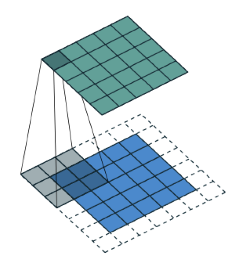 ::::
:::
::::
:::
Different types of layers in a CNN
::: columns :::: {.column width=50%} \small \textcolor{gray}{1. Convolutional layers} \newline \includegraphics[width=0.9\textwidth]{figures/cnn_conv_layer.png} :::: :::: {.column width=50%} \small \textcolor{gray}{3. Fully connected layers} \newline \includegraphics[width=0.9\textwidth]{figures/cnn_fully_connected.png} :::: :::
\vspace{3ex}
::: columns
:::: {.column width=60%}
\vfill
\small \textcolor{gray}{2. Pooling layers} \newline
\includegraphics[width=\textwidth]{figures/cnn_pooling.png}
::::
:::: {.column width=40%}
\textcolor{gray}{\footnotesize Afshine Amidi, Shervine Amidi}
\textcolor{gray}{\footnotesize Convolutional Neural Networks cheatsheet}
::::
:::
MNIST classification with a CNN in Keras
\footnotesize
from tensorflow.keras.models import Sequential
from tensorflow.keras.layers import Dense, Flatten, MaxPooling2D, Conv2D, Input

# conv layer with 8 3x3 filters
model = Sequential(
    [
        Input(shape=input_shape),
        Conv2D(8, kernel_size=(3, 3), activation="relu"),
        MaxPooling2D(pool_size=(2, 2)),
        Flatten(),
        Dense(16, activation="relu"),
        Dense(num_classes, activation="softmax"),
    ]
)

model.summary()
\normalsize
Defining the CNN in Keras (2)
\footnotesize
Model: "sequential_1"
_________________________________________________________________
Layer (type)                 Output Shape              Param #
=================================================================
conv2d_1 (Conv2D)            (None, 26, 26, 8)         80
_________________________________________________________________
max_pooling2d_1 (MaxPooling2 (None, 13, 13, 8)         0
_________________________________________________________________
flatten_1 (Flatten)          (None, 1352)              0
_________________________________________________________________
dense_2 (Dense)              (None, 16)                21648
_________________________________________________________________
dense_3 (Dense)              (None, 10)                170
=================================================================
Total params: 21,898
Trainable params: 21,898
Non-trainable params: 0
\normalsize
Model definition
Using Keras, you have to compile a model, which means adding the loss function, the optimizer algorithm and validation metrics to your training setup.
\vspace{5ex}
\footnotesize
model.compile(loss="categorical_crossentropy",
        optimizer="adam",
        metrics=["accuracy"])
\normalsize
Model training
\footnotesize
from tensorflow.keras.callbacks import ModelCheckpoint, EarlyStopping

checkpoint = ModelCheckpoint(
            filepath="mnist_keras_model.h5",
            save_best_only=True,
            verbose=1)
early_stopping = EarlyStopping(patience=2)

history = model.fit(x_train, y_train, # Training data
            batch_size=200, # Batch size
            epochs=50, # Maximum number of training epochs
            validation_split=0.5, # Use 50% of the train dataset for validation
            callbacks=[checkpoint, early_stopping]) # Register callbacks
\normalsize
Exercise 4: Training a digit-classification neural network on the MNIST dataset using Keras
\small \textcolor{gray}{05_neural_networks_ex_4_mnist_keras_train.ipynb} \normalsize
\vspace{5ex}
a) Plot training and validation loss as well as training and validation accuracy as a function of the number of epochs
b) Determine the accuracy of the fully trained model.
c) Create a second notebook that reads the trained model (mnist_keras_model.h5). Read your_own_digit.png and classify it. Create your own 28 \times 28 pixel digits with a program like gimp and check how the model performs.
Practical advice -- Which algorithm to choose?
\textcolor{gray}{From Kaggle competitions:}
\vspace{3ex} Structured data: "High level" features that have meaning:
- feature engineering + decision trees
- Random forests
- XGBoost
\vspace{3ex} Unstructured data: "Low level" features, no individual meaning:
- deep neural networks
- e.g. image classification: convolutional NN
Outlook: Autoencoders
::: columns :::: {.column width=50%}
- Unsupervised method based on neural networks to learn a representation of the input data
- Autoencoders learn to copy the input to the output layer
- low dimensional coding of the input in the central layer
- The decoder generates data based on the coding (generative model)
- Applications
- Dimensionality reduction
- Denoising of data
- Machine translation :::: :::: {.column width=50%} \vspace{3ex} \begin{center} \includegraphics[width=\textwidth]{figures/autoencoder_example.pdf} \end{center} :::: :::
Outlook: Generative adversarial network (GANs)
\begin{center} \includegraphics[width=0.65\textwidth]{figures/gan.png} \end{center} \scriptsize \textcolor{gray}{https://developers.google.com/machine-learning/gan/gan_structure} \normalsize
- Discriminator's classification provides a signal that the generator uses to update its weights
- Application in particle physics: fast detector simulation
- Full GEANT simulation usually very CPU intensive
The future
"Das Interessante an unserer Intelligenz ist, dass wir Go spielen können und dann vom Tisch aufstehen und Essen machen können, was eine Maschine nicht kann."
\vspace{2ex}
\color{gray} \small \hfill Bernhard Schölkopf, Max-Planck-Institut für intelligente Systeme (Interview FAZ) \normalsize \color{black}
\vfill
"My view is throw it all away and start again"
\color{gray} \small \hfill Geoffrey Hinton (DNN pioneer) on deep neural networks and backpropagation (Interview, 2017) \normalsize \color{black}