ML-Kurs-SS2023

Machine Learning Kurs im Rahmen der Studierendentage im SS 2023

21 KiB

Raw Blame History

% Introduction to Data Analysis and Machine Learning in Physics: \ 2. Data modeling and fitting % Day 1: 11. April 2023 % \underline{Jörg Marks}, Klaus Reygers

Data modeling and fitting - introduction

Data analysis is a process of understanding and modeling measured data. The goal is to find patterns and to obtain inferences allowing to observe underlying patterns.

There are 2 approaches to statistical data modeling
- Hypothesis testing: is our data compatible with a certain model?
- Determination of model parameter: use the data to determine the parameters of a (theoretical) model
For the determination of model parameter
- Analysis of data distributions $\rightarrow$ mean, variance, median, FWHM, .... \newline allows for an approximate determination of model parameter
- Data fitting with the least square method $\rightarrow$ an iterative process which minimizes the deviation of a model decribed by parameters from data. This determines the optimal values and uncertainties of the parameters.
- Maximum likelihood fitting $\rightarrow$ find a set of model parameters which most likely describe the data by maximizing the probability distributions.

The parameter determination by minimization is an integral part of machine learning approaches, here a system learns patterns and predicts related ones. This is the focus in the upcoming days.

Data modeling and fitting - introduction

Data analysis is a process of understanding and modeling measured data. The goal is to find patterns and to obtain inferences allowing to observe underlying patterns.

There are 2 approaches to statistical data modeling
- Hypothesis testing: is our data compatible with a certain model?
- Determination of model parameter: use the data to determine the parameters of a (theoretical) model
For the determination of model parameter
- Analysis of data distributions $\rightarrow$ mean, variance, median, FWHM, .... \newline allows for an approximate determination of model parameter
- \textcolor{blue}{Data fitting with the least square method $\rightarrow$ an iterative process which minimizes the deviation of a model decribed by parameters from data. This determines the optimal values and uncertainties of the parameters.}
- Maximum likelihood fitting $\rightarrow$ find a set of model parameters which most likely describe the data by maximizing the probability distributions.

The parameter determination by minimization is an integral part of machine learning approaches, here a system learns patterns and predicts related ones. This is the focus in the upcoming days.

Least Square (LS) Method (1)

The method determines the \textcolor{blue}{optimal parameters of functions to gaussian distributed measurements}.

Lets consider a sample of $n$ measurements $y_{i}$ and a parametrized description of the measurement $\eta_{i} = f(x_{i} | \theta)$ with a parameter set $\theta = \theta_{1}, \theta_{2} ,.... \theta_{k}$, dependent values $x_{i}$ and measurement errors $\sigma_{i}$.

The parameter set should be determined such that \begin{equation*} \color{blue}{S = \sum \limits_{i=1}^{n} \frac{(y_i-\eta_i)^2}{\sigma_i^2} = \sum \limits_{i=1}^{n} \frac{(y_i- f(x_i|\theta))^2}{\sigma_i^2} \longrightarrow , minimal } \end{equation*} In case of correlated measurements the covariance matrix of the $y_{i}$ has to be taken into account. This is accomplished by defining a weight matrix from the covariance matrix of the input data. A decorrelation of the input data should be considered. \vspace{0.2cm}

$S$ follows a $\chi^{2}$-distribution with $(n-k)$ degrees of freedom.

Least Square (LS) Method (2)

\setbeamertemplate{itemize item}{\color{red}\tiny$\blacksquare$}

Example LS-method \vspace{0.2cm}

Often the fit function $f(x, \theta)$ is linear in $\theta = \theta_{1}, \theta_{2} ,.... \theta_{k}$ \vspace{0.2cm}

$f(x | \theta) = \theta_{1} f_{1}(x) + .... + \theta_{k} f_{k}(x)$ \vspace{0.2cm}

If the model is a straight line and our parameters are $\theta_{1}$ and $\theta_{2}$ $(f_{1}(x) = 1,$ $f_{2}(x) = x)$ we have $f(x | \theta) = \theta_{1} + \theta_{2} x$ \vspace{0.2cm}

The LS equation is \vspace{0.2cm}

$\color{blue}{S = \sum \limits_{i=1}^{n} \frac{(y_i-\eta_i)^2}{\sigma_i^2} } \color{black} {= \sum \limits_{i=1}^{n} \frac{(y_{i} - \theta_{1} - x_{i} \theta_{2})^2}{\sigma_i^2 }}$ \hspace{0.4cm} and with \vspace{0.2cm}

$\frac{\partial S}{\partial \theta_1} = \sum\limits_{i=1}^{n} \frac{-2 (y_i - \theta_1 - x_i \theta_2)}{\sigma_i^2} = 0$ \hspace{0.4cm} and \hspace{0.4cm} $\frac{\partial S}{\partial \theta_2} = \sum\limits_{i=1}^{n} \frac{-2 x_i (y_i - \theta_1 - x_i \theta_2)}{\sigma_i^2} = 0$ \vspace{0.2cm}

the parameters $\theta_{1}$ and $\theta_{2}$ can be determined.

\vspace{0.2cm} \textcolor{olive}{In case of linear fit functions solutions can be found by matrix inversion}

\vfill

Least Square (LS) Method (3)

\setbeamertemplate{itemize item}{\color{red}\tiny$\blacksquare$}

Use of a nonlinear fit function $f(x, \theta)$ like \hspace{0.4cm} $f(x | \theta) = \theta_{1} \cdot e^{-\theta_{2} x}$ \vspace{0.2cm}

results in the LS equation \vspace{0.2cm}

$\color{blue}{S = \sum \limits_{i=1}^{n} \frac{(y_i-\eta_i)^2}{\sigma_i^2} } \color{black} {= \sum \limits_{i=1}^{n} \frac{(y_{i} - \theta_{1} \cdot e^{-\theta_{2} x_{i}})^2}{\sigma_i^2 }}$ \hspace{0.4cm} \vspace{0.2cm}

which we have to minimize \vspace{0.2cm}

$\frac{\partial S}{\partial \theta_1} = \sum\limits_{i=1}^{n} \frac{ 2 e^{-2 \theta_2 x_i} ( \theta_1 - y_i e^{\theta_2 x_i} )} {\sigma_i^2 } = 0$ \hspace{0.4cm} and \hspace{0.4cm} $\frac{\partial S}{\partial \theta_2} = \sum\limits_{i=1}^{n} \frac{ 2 \theta_1 x_I e^{-2 \theta_2 x_i} (y_i e^{\theta_2 x_i} - \theta_1)} {\sigma_i^2 } = 0$

\vspace{0.4cm}

In a nonlinear system, the LS Ansatz leads to derivatives which are functions of the independent variable and the parameters $\color{red}\rightarrow$ \textcolor{olive}{no closed solutions} \vspace{0.4cm}

In general, we have gradient equations which don't have closed solutions. There are a couple of methods including approximations which allow together with numerical methods to find a global minimum, Gauss–Newton algorithm, Levenberg–Marquardt algorithm, gradient descend methods and also direct search methods.

Minuit - a programm package for minimization (1)

In general data fitting and also solving machine learning algorithms lead to a minimization problem of functions. In the 1975-1980 F. James (CERN) developed a FORTRAN-based package, \textcolor{violet}{MINUIT}, which is a framework to handle multiparameter minimization and compute the best-fit parameter values and uncertainties, including correlations between the parameters. \vspace{0.2cm}

The user provides a minimization function $F(X,P)$ with the parameter space $P=(p_1,....p_k)$ and variable space $X$ (also multi-dimensional). There is an interface via functions which influences the minimization process. MINUIT provides \textcolor{violet}{error calculations} including correlations for the parameter space by evaluating the shape of the function in some neighbourhood of the minimum. \vspace{0.2cm}

The package has now a new object-oriented implementation as \textcolor{violet}{Minuit2 library} , written in C++. \vspace{0.2cm}

During the minimization $F(X,P)$ is evaluated for various $X$. For the choice of $P=(p_1,....p_k)$ different methods are used

Minuit - a programm package for minimization (2)

\vspace{0.4cm} \textcolor{olive}{SEEK}: Search for the minimum with Monte Carlo methods, mostly used at the start of the minimization with unknown starting values. It is not a converging algorithm. \vspace{0.2cm}

\textcolor{olive}{SIMPLX}: Uses the simplex method of Nelder and Mead. Function values are compared in the parameter space. Via step size control the minimum is approached. Parameter errors are only approximate, no covariance matrix is calculated. \vspace{0.2cm}

\textcolor{olive}{MIGRAD}: Uses an algorithm of R. Fletcher, which takes the function and the gradient to approach the minimum with a variable metric method. An error matrix and correlation coefficients are available \vspace{0.2cm}

\textcolor{olive}{HESSE}: Calculates the hessian matrix of second derivatives and determines the covariance matrix. \vspace{0.2cm}

\textcolor{olive}{MINOS}: Calculates (asymmetric) errors using likelihood profiles. The algorithm for finding the positive and negative MINOS errors for parameter $n$ consists of varying $n$ each time minimizing $F(X,P)$ with respect to all the others. \vspace{0.2cm}

Minuit - a programm package for minimization (3)

\vspace{0.4cm}

Fit process with the minuit package \vspace{0.2cm}

\setbeamertemplate{itemize item}{\color{red}\tiny$\blacksquare$}

The individual steps decribed above can be called several times and in different order during the minimization process.
Each of the parameters $p_i$ of $P=(p_1,....p_k)$ can be set constant and released during the minimization steps.
Problems are expected in models with strong correlation between parameters $\rightarrow$ change model to uncorrelated definitions
Local minima, edges/steps or undefined ranges in $F(X,P)$ are problematic $\rightarrow$ simplify your model

\vspace{3cm}

Minuit2 - The iminuit package

\vspace{0.4cm}

\textcolor{violet}{iminuit} is a Jupyter-friendly Python interface for the Minuit2 C++ library. \vspace{0.2cm}

\setbeamertemplate{itemize item}{\color{red}\tiny$\blacksquare$}

The class iminuit.Minuit instanciates the minuit object. The minimizer function is given as argument. Basic steering of the fit like setting start parameters, error definition and print level is also done here.

\footnotesize

     from iminuit import Minuit
     def fcn(x, y, z):                    # definition of the minimizer function
         return (x - 2) ** 2 + (y - x) ** 2 + (z - 4) ** 2
     fcn.errordef = Minuit.LEAST_SQUARES  # for Minuit to compute errors correctly
     m = Minuit(fcn, x=0, y=0, z=0)       # instanciate minuit, set start values

\normalsize

Several methods determine the interaction with the fitting process, calls to migrad, hesse or printing of parameters and errors

\footnotesize

     ......
     m.migrad()                     # run optimiser
     print(m.values , m.errors)     # print results
     m.hesse()                      # run covariance estimator

\normalsize

Minuit2 - iminuit example

\vspace{0.2cm}

\setbeamertemplate{itemize item}{\color{red}\tiny$\blacksquare$}

The function fcn describes the model with parameters to be determined by data. fcn is minimal when the model parameters agree best with data. fcn has positional arguments, one for each fit parameter. iminuit example fit:

\textcolor{violet}{02_fit_exp_fit_iMinuit.ipynb}

\footnotesize

     ......
     x =  np.array([....],dtype='d') # measurements x
     y =  np.array([....],dtype='d') # measurements y
     dy = np.array([....],dtype='d') # error in y
     def xp(a, b , c):
         return a * np.exp(b*x) + c
     # least-squares function = sum of data residuals squared
     def fcn(a,b,c):
        return np.sum((y - xp(a,b,c)) ** 2 / dy ** 2)
     # limit the range of b and fix parameter c
     m = Minuit(fcn,a=1,b=-0.7,c=1)
     m.migrad()                      # run minimizer
     m.fixed["c"] = True             # fix or release  parameter c
     m.migrad()                      # rerun minimizer
     # Might be useful to fix parameters or limit the range for some applications

\normalsize

Minuit2 - iminuit (3)

\vspace{0.2cm}

\setbeamertemplate{itemize item}{\color{red}\tiny$\blacksquare$}

Results and control information of the fit can be printed and accessed in the the prorgamm.

\footnotesize

     ......
     m = Minuit(fcn,....)               # run the initializer
     m.migrad()                         # run minimizer
     a_fit = m.values['a']              # get parameter value a
     a_fit_error =  m.errors['a']       # get parameter error of a
     print (m.values,m.errors)          # print results

\normalsize

After processing Hesse, covariance and correlation information of the fit is available

\footnotesize

     ......
     m.hesse()                           # run covariance estimator
     m.matrix()                          # get covariance matrix
     m.matrix(correlation=True)          # get full correlation matrix
     cov = m.np_matrix()                 # save matrix to numpy
     cor = m.np_matrix(correlation=True) 
     print(cor[0, 1])      # print correlation between parameter 1 and 2

\normalsize

Minuit2 - iminuit (4)

\setbeamertemplate{itemize item}{\color{red}\tiny$\blacksquare$}

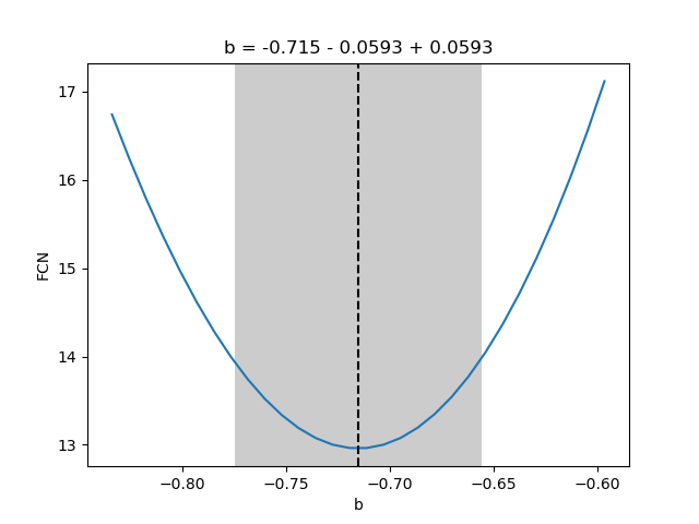
Minos provides asymmetric uncertainty intervals and parameter contours by scanning one parameter and minimizing the function with respect to all other parameters for each scan point. Results are displayed with matplotlib.

\footnotesize

     ......
     m.minos()
     print (m.get_merrors()['a'])
     m.draw_profile('b')
     m.draw_mncontour('a', 'b', cl=[1, 2, 3, 4])

::: columns :::: {.column width=40%} :::: :::: {.column width=40%} :::: :::

Exercise 3

Plot the following data with matplotlib as in the iminuit example:

\footnotesize

   x:   0.2,0.4,0.6,0.8,1.,1.2,1.4,1.6,1.8,2.,2.2,2.4,2.6,2.8,3.,3.2,
        3.4,3.6, 3.8,4.
   y:   0.04,0.021,0.035,0.03,0.029,0.019,0.024,0.018,0.019,0.022,0.02,
        0.025,0.018,0.024,0.019,0.021,0.03,0.019,0.03,0.024
   dy:  1.792,1.695,1.541,1.514,1.427,1.399,1.388,1.270,1.262,1.228,1.189,
        1.182,1.121,1.129,1.124,1.089,1.092,1.084,1.058,1.057

\normalsize \setbeamertemplate{itemize item}{\color{red}$\square$}

Exchange in the example iminuit fit 02_fit_exp_fit_iMinuit.ipynb the exponential function by a 3rd order polynomial and perform the fit
Compare the correlation of the parameters of the exponential and the polynomial fit
What defines the fit quality, give an estimate

\small Solution: \textcolor{violet}{02_fit_ex_3_sol.ipynb} \normalsize

Exercise 4

Plot the following data with matplotlib:

\footnotesize

   x:   1, 2, 3, 4, 5, 6, 7, 8, 9, 10
   dx:  0.1,0.1,0.5,0.1,0.5,0.1,0.5,0.1,0.5,0.1
   y:   1.1,2.3,2.7,3.2,3.1,2.4,1.7,1.5,1.5,1.7
   dy:  0.15,0.22,0.29,0.39,0.31,0.21,0.13,0.15,0.19,0.13

\normalsize \setbeamertemplate{itemize item}{\color{red}$\square$}

Perform a fit with iminuit. Which model do you use?
Plot the resulting fit function in the graph with the data
Print the covariance matrix. Can we improve the errors.
Can you draw a contour plot of 2 of the fit parameters.

\small Solution: \textcolor{violet}{02_fit_ex_4_sol.ipynb} \normalsize

PyROOT

\textcolor{violet}{PyROOT} is the python binding for the C++ data analysis toolkit \textcolor{violet}{ROOT} developed with and for the LHC community. You can access the full ROOT functionality from Python while benefiting from the performance of the ROOT C++ libraries. The PyROOT bindings are automatic and dynamic and are able to interoperate with widely-used Python data-science libraries as NumPy, pandas, SciPy scikit-learn and tensorflow.

ROOT/PyROOT can be installed easily within anaconda3 (ROOT version 6.26.06 or later ) or is available in the \textcolor{violet}{CIP jupyter3 Hub}
Tools for statistical analysis, a math library with optimized algorithms, multivariate analysis, visualization and simulation of data.
Storing data including objects and classes with compression in files is a very powerfull aspect for any data analysis project
Within PyROOT Minuit2 can be accessed easily either with predefined functions or your own function definition
For advanced statistical analyses and data modeling likelihood fitting with the packages rooFit and rooStats is available.

Example reading the invariant mass measurements of a $D^0$ from a text file and determine $\mu$ and $\sigma$ \hspace{1.0cm} \small \textcolor{violet}{02_fit_histFit.ipynb} \hspace{0.5cm} run with: python3 -i 02_fit_histFit.py \normalsize

\footnotesize

     import numpy as np
     import math
     from ROOT import TCanvas, TFile, TH1D, TF1, TMinuit, TFitResult
     data = np.genfromtxt('D0Mass.txt', dtype='d') # read data from text file
     c = TCanvas('c','D0 Mass',200,10,700,500)     # instanciate output canvas
     d0 = TH1D('d0','D0 Mass',200,1700.,2000.)     # instanciate histogramm
     for x in data :                               # fill data into histogramm d0
          d0.Fill(x)
     def pyf_tf1_params(x, p):                     # define fit function
          return p[0] * math.exp (-0.5 * ((x[0] - p[1])**2 / p[2]**2))
     func = TF1("func",pyf_tf1_params,1840.,1880.,3)
     # func = TF1("func",'gaus',1840.,1880.)  # use predefined function   
     func.SetParameters(500.,1860.,5.5)    # set start parameters
     myfit = d0.Fit(func,"S")              # fit function to the histogramm data
     print ("Fit results: mean=",myfit.Parameter(0)," +/- ",myfit.ParError(0))
     c.Draw()                                      # draw canvas
     myfile = TFile('myOutFile.root','RECREATE')   # Open a ROOT file for output
     c.Write()                                     # Write canvas
     d0.Write()                                    # Write histogram
     myfile.Close()                                # close file

\normalsize

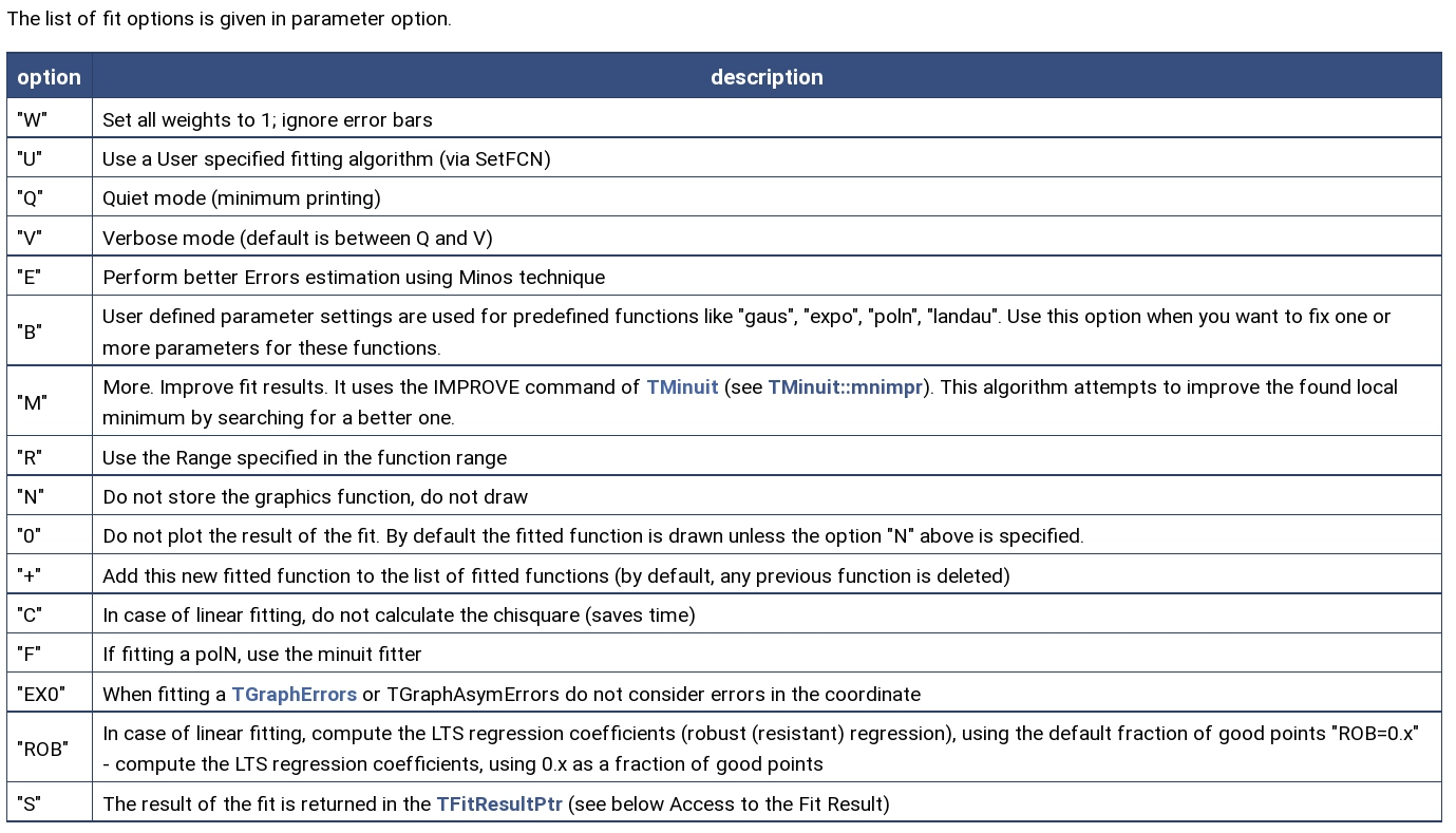
Fit Options \vspace{0.1cm}

::: columns :::: {.column width=2%} :::: :::: {.column width=98%} :::: :::

Exercise 5

Read text file \textcolor{violet}{FitTestData.txt} and draw a histogramm using PyROOT. \setbeamertemplate{itemize item}{\color{red}$\square$}

Determine the mean and sigma of the signal distribution. Which function do you use for fitting?
The option S fills the result object.
Try to improve the errors of the fit values with minos using the option E and also try the option M to scan for a new minimum, option V provides more output.
Fit the background outside the signal region use the option R+ to add the function to your fit

\small Solution: \textcolor{violet}{02_fit_ex_5_sol.ipynb} \normalsize

iPython Examples for Fitting

The different python packages are used in \textcolor{blue}{example iPython notebooks} to demonstrate the fitting of a third order polynomial to the same data available as numpy arrays.

\setbeamertemplate{itemize item}{\color{red}\tiny$\blacksquare$}

LSQ fit of a polynomial to data using Minuit2 with \textcolor{blue}{iminuit} and \textcolor{blue}{matplotlib} plot:

\small \textcolor{violet}{02_fit_iminuitFit.ipynb} \normalsize
Graph fitting with \textcolor{blue}{pyROOT} with options using a python function including confidence level plot:

\small \textcolor{violet}{02_fit_fitGraph.ipynb} \normalsize
Graph fitting with \textcolor{blue}{numpy} and confidence level plotting with \textcolor{blue}{matplotlib}:

\small \textcolor{violet}{02_fit_numpyFit.ipynb}
\normalsize
Graph fitting with a polynomial fit of \textcolor{blue}{scikit-learn} and plotting with \textcolor{blue}{matplotlib}:

\normalsize \small \textcolor{violet}{02_fit_scikitFit.ipynb} \normalsize

21 KiB Raw Blame History

Data modeling and fitting - introduction

Data modeling and fitting - introduction

Least Square (LS) Method (1)

Least Square (LS) Method (2)

Least Square (LS) Method (3)

Minuit - a programm package for minimization (1)

Minuit - a programm package for minimization (2)

Minuit - a programm package for minimization (3)

Minuit2 - The iminuit package

Minuit2 - iminuit example

Minuit2 - iminuit (3)

Minuit2 - iminuit (4)

Exercise 3

Exercise 4

PyROOT

Exercise 5

iPython Examples for Fitting

21 KiB

Raw Blame History