35 KiB
| title | author | date |
|---|---|---|
| | Introduction to Data Analysis and Machine Learning in Physics: | 3. Machine Learning Basics | Martino Borsato, Jörg Marks, Klaus Reygers | Studierendentage, 11-14 April 2022 |
Exercises
- Exercise 1: Air shower classification (MAGIC telescope)
- Logistic regression
03_ml_basics_ex01_magic.ipynb
- Exercise 2: Hand-written digit recognition with logistic regression
- Logistic regression
03_ml_basics_ex02_mnist_softmax_regression.ipynb
- Exercise 3: Data preprocessing
What is machine learning? (1)

What is machine learning? (2)
"Machine learning is the subfield of computer science that gives computers the ability to learn without being explicitly programmed" -- Wikipedia
\vspace{2ex} Example: spam detection \hfill \scriptsize \textcolor{gray}{J. Mayes, Machine learning 101} \normalsize
\begin{center} \includegraphics[width=0.9\textwidth]{figures/ml_example_spam.png} \vspace{2ex}
Manual feature engineering vs. automatic feature detection \end{center}
AI, ML, and DL
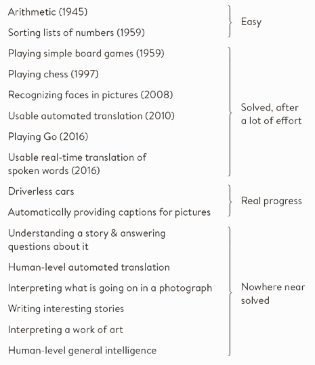
"AI is the study of how to make computers perform things that, at the moment, people do better."
\tiny \textcolor{gray}{Elaine Rich, Artificial intelligence, McGraw-Hill 1983} \normalsize
\vfill
\tiny \hfill \textcolor{gray}{G. Marcus, E. Davis, Rebooting AI} \normalsize
\begin{figure}
\centering
%
\vfill "deep" in deep learning: artificial neural nets with many neurons and multiple layers of nonlinear processing units for feature extraction
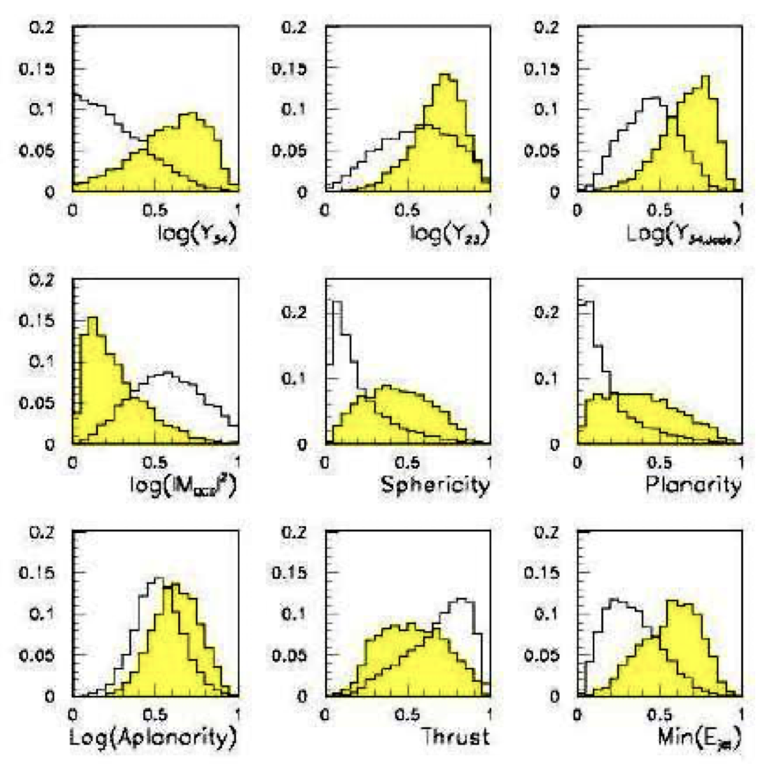
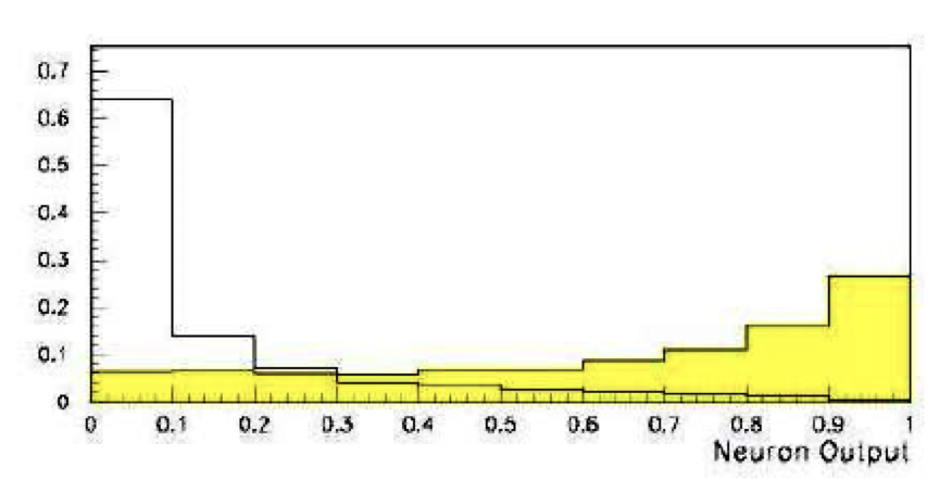
Multivariate analysis: An early example from particle physics
::: columns
:::: {.column width=55%}
 {width=99%}
::::
:::: {.column width=45%}
{width=99%}
::::
:::: {.column width=45%}
- Signal: $e^+e^- \to W^+W^-$
- often 4 well separated hadron jets
- Background: $e^+e^- \to qqgg$
- 4 less well separated hadron jets
- Input variables based on jet structure, event shape, ... none by itself gives much separation.
 {width=85%}
\tiny \textcolor{gray}{(Garrido, Juste and Martinez, ALEPH 96-144)} \normalsize
::::
:::
{width=85%}
\tiny \textcolor{gray}{(Garrido, Juste and Martinez, ALEPH 96-144)} \normalsize
::::
:::
Applications of machine learning in physics
- Particle physics: Particle identification / classification
- Astronomy: Galaxy morphology classification
- Chemistry and material science: predict properties of new molecules / materials
- Many-body quantum matter: classification of quantum phases
\vspace{3ex} \scriptsize \textcolor{gray}{Machine learning and the physical sciences, arXiv:1903.10563} \normalsize
Some successes and unsolved problems in AI
::: columns
:::: {.column width=50%}
 {width=85%}
\tiny \textcolor{gray}{M. Woolridge, The road to conscious machines} \normalsize
:::: :::: {.column width=50%}
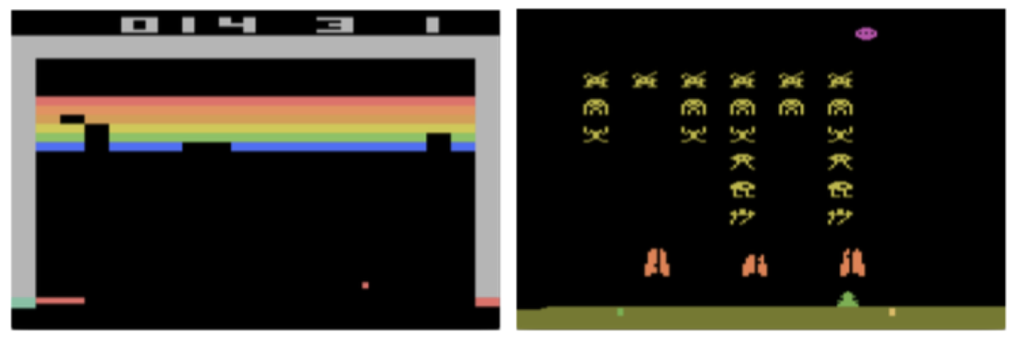
Impressive progress in certain fields:
\small
- Image recognition
- Speech recognition
- Recommendation systems
- Automated translation
- Analysis of medical data \normalsize \vfill
How can we profit from these developments in physics? :::: :::
The deep learning hype -- why now?
Artificial neural networks are around for decades. Why did deep learning take off after 2012?
\vspace{5ex}
- Improved hardware -- graphical processing units [GPUs]
- Large data sets (e.g. images) distributed via the Internet
- Algorithmic advances
Different modeling approaches
- Simple mathematical representation like linear regression. Favored by statisticians.
- Complex deterministic models based on scientific understanding of the physical process. Favored by physicists.
- Complex algorithms to make predictions that are derived from a huge number of past examples (“machine learning” as developed in the field of computer science). These are often black boxes.
- Regression models that claim to reach causal conclusions. Used by economists.
\tiny \textcolor{gray}{D. Spiegelhalter, The Art of Statistics – Learning from data} \normalsize
Machine learning: The "hello world" problem
::: columns :::: {.column width=45%}
Recognition of handwritten digits
- MNIST database (Modified National Institute of Standards and Technology database)
- 60,000 training images and 10,000 testing images labeled with correct answer
- 28 pixel x 28 pixel
- Algorithms have reached "near-human performance"
- Smallest error rate (2018): 0.18%
::::
:::: {.column width=55%}
\tiny \color{gray}{\texttt{https://en.wikipedia.org/wiki/MNIST_database}} \normalsize
:::: :::
Machine learning: Image recognition
ImageNet database
- 14 million images, 22,000 categories
- Since 2010, the annual ImageNet Large Scale Visual Recognition Challenge (ILSVRC): 1.4 million images, 1000 categories
- In 2017, 29 of 38 competing teams got less than 5% wrong
\begin{figure} \centering \includegraphics[width=0.8\textwidth]{figures/imagenet.png} \end{figure}
ImageNet: Large Scale Visual Recognition Challenge
\begin{figure} \centering \includegraphics[width=0.8\textwidth]{figures/imagenet_challenge.png} \end{figure}
\vfill
\scriptsize \textcolor{gray}{O. Russakovsky et al, arXiv:1409.0575} \normalsize
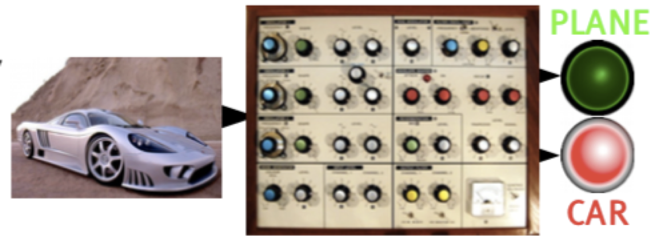
Adversarial attack
\begin{figure} \centering \includegraphics[width=\textwidth]{figures/adversarial_attack.png} \end{figure}
\vspace{3ex} \scriptsize \textcolor{gray}{Ian J. Goodfellow, Jonathon Shlens, Christian Szegedy, arXiv:1412.6572v1} \normalsize
Types of machine learning
::: columns :::: {.column width=60%} Reinforcement learning
\small
- The machine ("the agent") predicts a scalar reward given once in a while
- Weak feedback \normalsize
::::
:::: {.column width=35%}
\tiny \textcolor{gray}{LeCun 2018, Power And Limits of Deep Learning} \normalsize
 ::::
:::
\vfill
::: columns
:::: {.column width=60%}
::::
:::
\vfill
::: columns
:::: {.column width=60%}
\vspace{1em} Supervised learning
\small
- The machine predicts a category based on labeled training data
- Medium feedback
\normalsize
::::
:::: {.column width=35%}
 ::::
:::
\vfill
::: columns
:::: {.column width=60%}
::::
:::
\vfill
::: columns
:::: {.column width=60%}
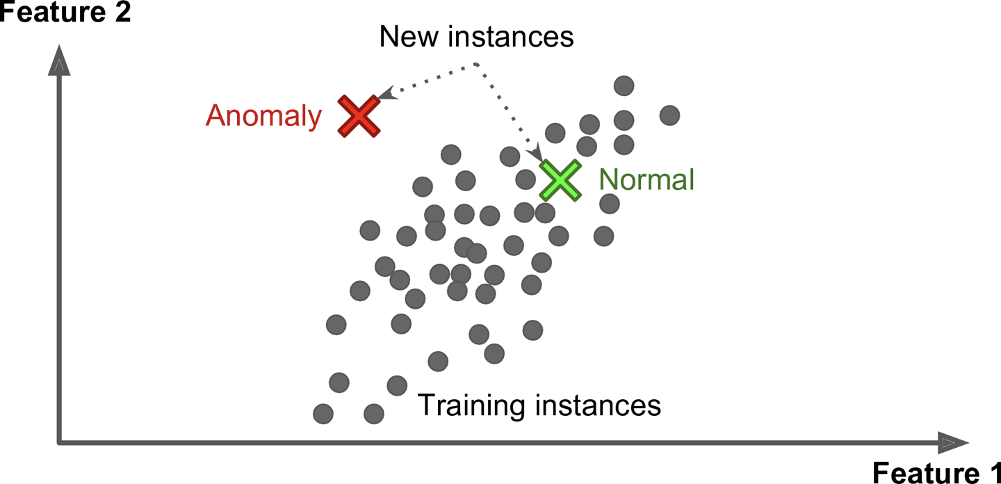
\vspace{1em} Unsupervised learning
\small
- Describe/find hidden structure from "unlabeled" data
- Cluster data in different sub-groups with similar properties
\normalsize
::::
:::: {.column width=35%}
 ::::
:::
::::
:::
Books on machine learning (1)
::: columns :::: {.column width=85%} Ian Goodfellow and Yoshua Bengio and Aaron Courville, \textit{Deep Learning}, free online http://www.deeplearningbook.org/
\vspace{8ex}
Kevin Murphy, \textit{Probabilistic Machine Learning: An Introduction}, draft pdf version
\vspace{7ex}
Aurelien Geron, \textit{Hands-On Machine Learning with Scikit-Learn and TensorFlow}
::::
:::: {.column width=15%}
 {width=65%}
\vspace{3ex}
 {width=65%}
\vspace{3ex}
 {width=65%}
:::: :::
Books on machine learning (2)
::: columns :::: {.column width=85%} Francois Chollet, \textit{Deep Learning with Python}
\vspace{10ex}
Martin Erdmann, Jonas Glombitza, Gregor Kasieczka, Uwe Klemradt, \textit{Deep Learning for Physics Research}
::::
:::: {.column width=15%}
 {width=65%}
\vspace{3ex}
 {width=65%}
:::: :::
Papers
A high-bias, low-variance introduction to Machine Learning for physicists
https://arxiv.org/abs/1803.08823
\vspace{3ex}
Machine learning and the physical sciences
https://arxiv.org/abs/1903.10563
Supervised learning in a nutshell
- Supervised Machine Learning requires labeled training data, i.e., a training sample where for each event it is known whether it is a signal or background event.
- Each event is characterized by $n$ observables: $\vec x = (x_1, x_2, ..., x_n) ;$ \textcolor{gray}{"feature vector"}
\begin{figure} \centering \raisebox{-0.5\height}{\includegraphics[width=0.69\textwidth]{figures/supervised_nutshell.png}} \raisebox{-0.5\height}{\includegraphics[width=0.30\textwidth]{figures/loss_fct.png}} \end{figure}
- Design function $y(\vec x, \vec w)$ with adjustable parameters $\vec w$
- Design a loss function
- Find best parameters which minimize loss
Supervised learning: classification and regression
The codomain $Y$ of the function y: $X \to Y$ can be a set of labels or classes or a continuous domain, e.g., $\mathbb{R}$
\vfill
- $Y$ = finite set of labels $\quad \to \quad$ \textcolor{red}{classification}
- binary classification: $Y = {0,1}$
- multi-class classification: $Y = {c_1, c_2, ..., c_n}$
- $Y$ = real numbers $\quad \to \quad$ \textcolor{red}{regression}
\vfill
\textcolor{gray}{"All the impressive achievements of deep learning amount to just curve fitting" \[0.5cm]} \footnotesize \textcolor{gray}{J. Pearl, Turing Award Winner 2011\} \tiny \color{gray}{To Build Truly Intelligent Machines, Teach Them Cause and Effect, Quantamagazine} \normalsize
Classification: Learning decision boundaries
\begin{figure} \centering \includegraphics{figures/decision_boundaries.png} \end{figure}
Supervised learning: Training, validation, and test sample
- Decision boundary fixed with \textcolor{blue}{training sample}
- Performance on training sample becomes better with more iterations
- Danger of overtraining: Statistical fluctuations of the training sample will be learnt
- \textcolor{blue}{Validation sample} = independent labeled data set not used for training $\rightarrow$ check for overtraining
- Sign of overtraining: performance on validation sample becomes worse $\rightarrow$ Stop training when signs of overtraining are observed (early stopping)
- Performance: apply classifier to independent \textcolor{blue}{test sample}
- Often: test sample = validation sample (only small bias)
Supervised learning: Cross validation
Rule of thumb if training data not expensive
::: columns :::: {.column width=60%}
- Training sample: 50%
- Validation sample: 25%
- Test sample: 25%
\vspace{2ex}
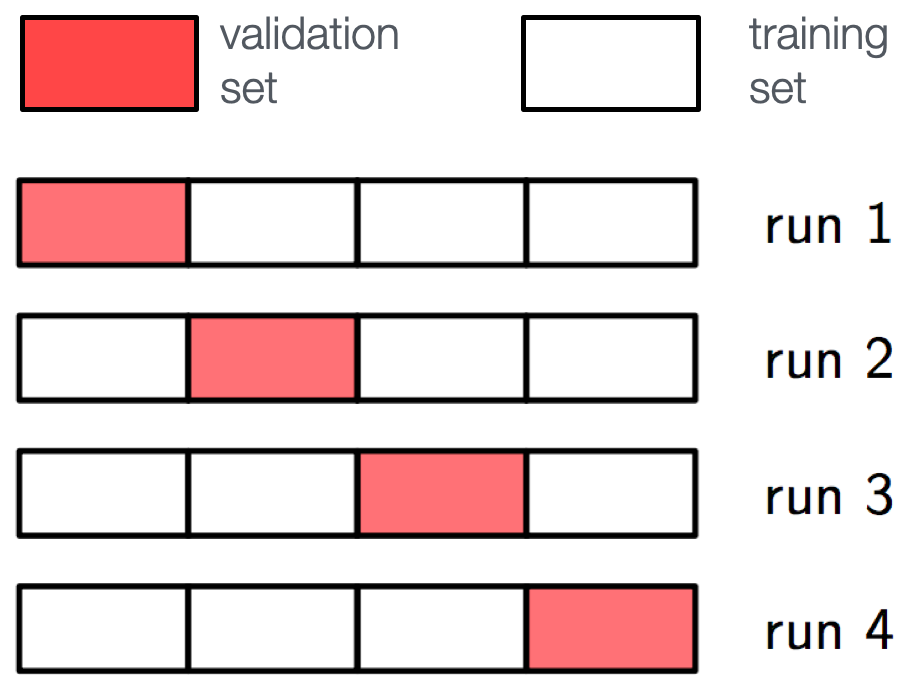
Cross validation (efficient use of scarce training data)
- Split training sample in $k$ independent subset $T_k$ of the full sample $T$
- Train on $T \setminus T_k$ resulting in $k$ different classifiers
- For each training event there is one classifier that didn't use this event for training
- Validation results are then combined :::: :::: {.column width=40%} \textcolor{gray}{Often test sample = validation sample (bias is rather small)}
\vspace{10ex}
 ::::
:::
::::
:::
Often used loss functions
::: columns :::: {.column width=45%} \textcolor{blue}{Square error loss}:
- often used in regression
:::: :::: {.column width=55%} $$ E(y(\vec x, \vec w), t) = (y(\vec x, \vec w) - t)^2 $$ :::: :::
\vfill
::: columns :::: {.column width=45%} \textcolor{blue}{Cross entropy}:
- $t \in {0,1}$
- $y(\vec x, \vec w)$: predicted probability for outcome $t=1$
- often used in classification
:::: :::: {.column width=55%} \begin{align*} E(y(\vec x, \vec w), t) = & - t \log y(\vec x, \vec w) \ & - (1 - t) \log(1 - y(\vec x, \vec w)) \end{align*}
:::: :::
More on entropy
- Self-information of an event $x$: $I(x) = - \log p(x)$
- in units of nats (1 nat = information gained by observing an event of probability $1/e$)
\vfill
- Shannon entropy: $H(P) = - \sum p_i \log p_i$
- Expected amount of information in an event drawn from a distribution $P$
- Measure of the minimum of amount of bits needed on average to encode symbols drawn from a distribution
\vfill
- Cross entropy: $H(P,Q) = - E[\log Q] = - \sum p_i \log q_i$
- Can be interpreted as a measure of the amount of bits needed when a wrong distribution Q is assumed while the data actually follows a distribution P
- Measure of dissimilarity between distributions P and Q (i.e, a measure of how well the model Q describes the true distribution P)
Hypothesis testing
::: columns :::: {.column width=55%} \includegraphics[width=\textwidth]{figures/signal_background_distr.png} :::: :::: {.column width=45%} \vspace{2ex} test statistic
- a (usually scalar) variable which is a function of the data alone that can be used to test hypotheses
- example: $\chi^2$ w.r.t. a theory curve
:::: :::
\textcolor{gray}{$\epsilon_\mathrm{B} \equiv \alpha$}: "background efficiency", i.e., prob. to misclassify bckg. as signal
\textcolor{gray}{$\epsilon_\mathrm{S} \equiv 1 - \beta$}: "signal efficiency"
\begin{center}
\begin{tabular}{ l l l}
& $H_0$ is true & $H_0$ is false (i.e., $H_1$ is true)\
\hline
$H_0$ is rejected & Type I error ($\alpha$) & Correct decision ($1 - \beta$) \
$H_0$ is not rejected & Correct decision ($1 - \alpha$) & Type II error ($\beta$) \
\hline
\end{tabular}
\end{center}
Neyman-Pearson Lemma
The likelihood ratio
$$ t(\vec x) = \frac{f(\vec x|H_1)}{f(\vec x|H_0)} $$
is an optimal test statistic, i.e., it provides highest "signal efficiency" $1-\beta$ for a given "background efficiency" $\alpha$. Accept hypothesis if $t(\vec x) > c$.
\vfill
Problem: the underlying pdf's are almost never known explicitly.
\vfill
Two approaches
-
Estimate signal and background pdf's and construct test statistic based on Neyman-Pearson lemma
-
Decision boundaries determined directly without approximating the pdf's (linear discriminants, decision trees, neural networks, ...)
Estimating PDFs from Histograms?
\begin{center} \includegraphics[width=0.8\textwidth]{figures/pdf_from_2d_histogram.png} $\color{gray} \text{approximate PDF by} ; N(x,y|S) ; \text{and} ; N(x,y|B)$ \end{center}
$M$ bins per variable in $d$ dimensions: $M^d$ cells$\to$ hard to generate enough training data (often not practical for $d > 1$)
In general in machine learning, problems related to a large number of dimensions of the feature space are referred to as the \textcolor{red}{"curse of dimensionality"}
Na$\text{"i}$ve Bayesian Classifier (also called "Projected Likelihood Classification")
Application of the Neyman-Pearson lemma (ignoring correlations between the $x_i$):
$$ f(x_1, x_2, ..., x_n) \quad \mbox{approximated as} \quad L = f_1(x_1) \cdot f_2(x_2) \cdot ... \cdot f_n(x_n) $$
\begin{align*}
\mbox{where} \quad
f_1(x_1) & = \int \mathrm dx_2 \mathrm dx_3 ... \mathrm dx_n; f(x_1, x_2, ..., x_n) \
f_2(x_2) & = \int \mathrm dx_1 \mathrm dx_3 ... \mathrm dx_n; f(x_1, x_2, ..., x_n) \
\vdots
\end{align*}
Classification of feature vector $x$:
$$
y(\vec x) = \frac{L_\mathrm{s}(\vec x)}{L_\mathrm{s}(\vec x) + L_\mathrm{b}(\vec x)} = \frac{1}{1 + L_\mathrm{b}(\vec x) / L_\mathrm{s}(\vec x)}
$$
Performance not optimal if true PDF does not factorize
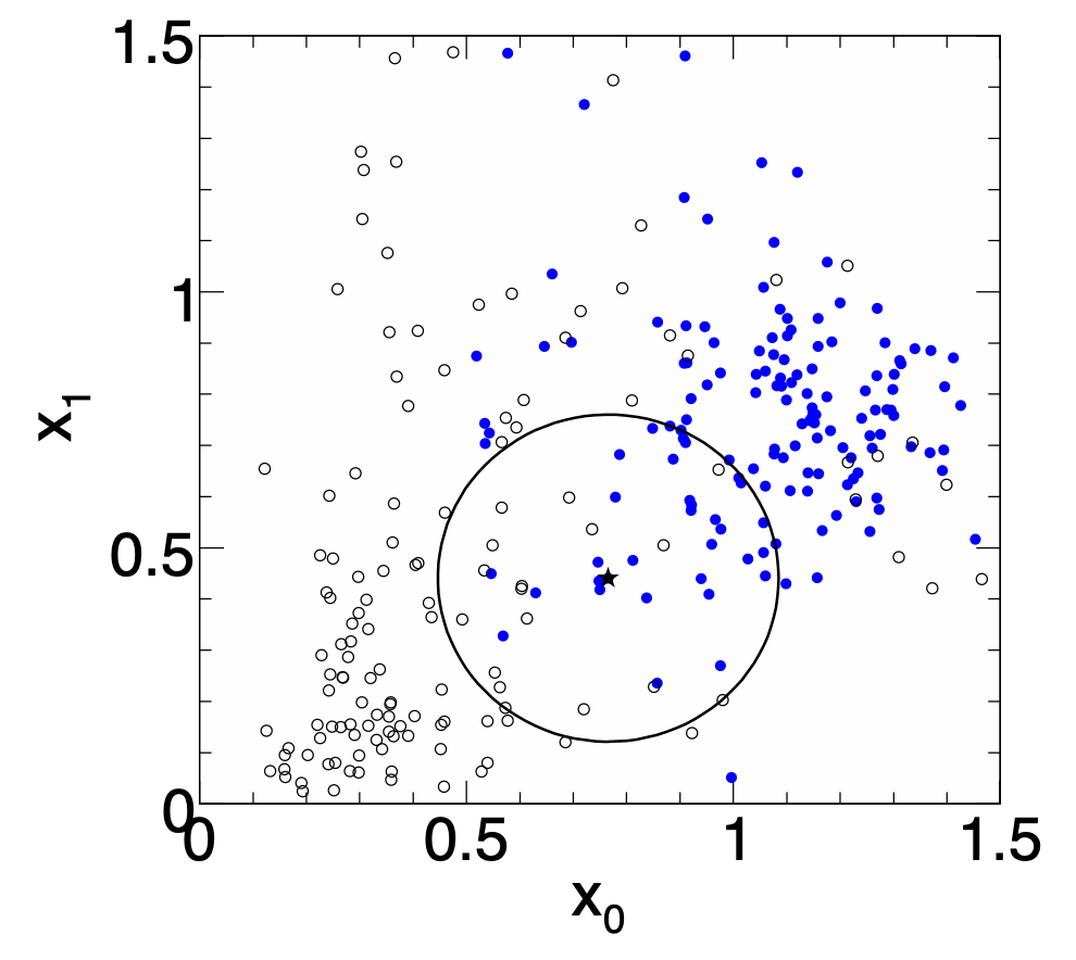
k-Nearest Neighbor Method (1)
$k$-NN classifier:
- Estimates probability density around the input vector
- $p(\vec x|S)$ and $p(\vec x|B)$ are approximated by the number of signal and background events in the training sample that lie in a small volume around the point $\vec x$
\vspace{2ex}
Algorithms finds $k$ nearest neighbors: $$ k = k_s + k_b $$
Probability for the event to be of signal type:
$$ p_s(\vec x) = \frac{k_s(\vec x)}{k_s(\vec x) + k_b(\vec x)} $$
k-Nearest Neighbor Method (2)
::: columns :::: {.column width=60%} Simplest choice for distance measure in feature space is the Euclidean distance: $$ R = |\vec x - \vec y|$$
Better: take correlations between variables into account:
$$ R = \sqrt{(\vec{x}-\vec{y})^T \mat{V}^{-1} (\vec{x}-\vec{y})} $$ $$ \mat{V} = \text{covariance matrix}, R = \text{"Mahalanobis distance"}$$
::::
:::: {.column width=40%}
 ::::
:::
::::
:::
\vfill
The $k$-NN classifier has best performance when the boundary that separates signal and background events has irregular features that cannot be easily approximated by parametric learning methods.
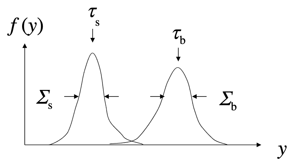
Fisher Linear Discriminant
Linear discriminant is simple. Can still be optimal if amount of training data is limited.
Ansatz for test statistic: $$ y(\vec x) = \sum_{i=1}^n w_i x_i = \vec w^\intercal \vec x $$
Choose parameters $w_i$ so that separation between signal and background distribution is maximum.
\vfill
Need to define "separation".
::: columns
:::: {.column width=45%}
\begin{center}
Fisher: maximize $$ J(\vec w) = \frac{(\tau_s - \tau_b)^2}{\Sigma_s^2 + \Sigma_b^2} $$
\end{center}
::::
:::: {.column width=55%}
 ::::
:::
::::
:::
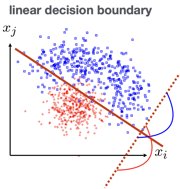
Fisher Linear Discriminant: Determining the Coefficients $w_i$
::: columns :::: {.column width=60%} Coefficients are obtained from: $$ \frac{\partial J}{\partial w_i} = 0 $$
\vspace{2ex}
Linear decision boundaries
\vspace{5ex}
Weight vector $\vec w$ can be interpreted as a direction in feature space onto which the events are projected.
::::
:::: {.column width=40%}
 ::::
:::
::::
:::
Linear regression revisited
\vfill
::: columns
:::: {.column width=50%}
\small \textcolor{gray}{"Galton family heights data": \ origin of the term "regression"} \normalsize

:::: :::: {.column width=50%}
- data: ${x_i,y_i}$ \
- objective: predict $y = f(x)$
- model: $f(x; \vec \theta) = m x + b, \quad \vec \theta = (m, b)$
- loss function: $J(\theta|x,y) = \frac{1}{N} \sum_{i=1}^N (y_i - f(x_i))^2$
- model training: optimal parameters $\hat{\vec{\theta}} = \mathrm{arg,min} , J(\vec \theta)$
:::: :::
Linear regression
-
Data: vectors with $p$ components ("features"): $\vec x = (x_1, ..., x_p)$
-
$n$ observations: ${\vec x_i, y_i}, \quad i = 1, ..., n$
-
Prediction for given vector $x$: $$ y = w_0 + w_1 x_1 + w_2 x_2 + ... + w_p x_p \equiv \vec w^\intercal \vec x \quad \text{where } x_0 := 1 $$
-
Find weights that minimze loss function: $$\hat{\vec{w}} = \underset{\vec w}{\min} \sum_{i=1}^{n} (\vec w^\intercal \vec x_i - y_i)^2$$
-
In case of linear regression closed-form solution exists: $$ \hat{\vec{w}} = (\mat{X}^\intercal \mat{X})^{-1} \mat{X}^\intercal \vec y \quad \text{where} ; X \in \mathbb{R}^{n \times p}$$
-
$X$ is called the design matrix, row $i$ of $X$ is $\vec x_i$
Linear regression with regularization
::: columns :::: {.column width=45%}
-
Standard loss function $$ C(\vec w) = \sum_{i=1}^{n} (\vec w^\intercal \vec x_i - y_i)^2 $$
-
Ridge regression $$ C(\vec w) = \sum_{i=1}^{n} (\vec w^\intercal \vec x_i - y_i)^2 + \lambda |\vec w|^2$$
-
LASSO regression $$ C(\vec w) = \sum_{i=1}^{n} (\vec w^\intercal \vec x_i - y_i)^2 + \lambda |\vec w| $$
:::: :::: {.column width=55%}
\vfill

Logistic regression (1)
- Consider binary classification task, e.g., $y_i \in {0,1}$
- Objective: Predict probability for outcome $y=1$ given an observation $\vec x$
- Starting with linear "score" $$ s = w_0 + w_1 x_1 + w_2 x_2 + ... + w_p x_p \equiv \vec w^\intercal \vec x$$
- Define function that translates $s$ into a quantity that has the properties of a probability $$ \sigma(s) = \frac{1}{1+e^{-s}} $$
- We would like to determine the optimal weights for a given training data set. They result from the maximum-likelihood principle.
Logistic regression (2)
- Consider feature vector $\vec x$. For a given set of weights $\vec w$ the model predicts
- a probability $p(1|\vec w) = \sigma(\vec w^\intercal \vec x)$ for outcome $y=1$
- a probabiltiy $p(0|\vec w) = 1 - \sigma(\vec w^\intercal \vec x)$ for outcome $y=0$
- The probability $p(y_i | \vec w)$ defines the likelihood $L_i(\vec w) = p(y_i | \vec w)$ (the likelihood is a function of the parameters $\vec w$ and the observations $y_i$ are fixed).
- Likelihood for the full data sample ($n$ observations) $$ L(\vec w) = \prod_{i=1}^n L_i(\vec w) = \prod_{i=1}^n \sigma(\vec w^\intercal \vec x)^{y_i} ,(1-\sigma(\vec w^\intercal \vec x))^{1-y_i} $$
- Maximizing the log-likelihood $\ln L(\vec w)$ corresponds to minimizing the loss function $$ C(\vec w) = - \ln L(\vec w) = \sum_{i=1}^n - y_i \ln \sigma(\vec w^\intercal \vec x) - (1-y_i) \ln(1-\sigma(\vec w^\intercal \vec x))$$
- This is nothing else but the cross-entropy loss function
scikit-learn
::: columns :::: {.column width=70%}
- Free software machine learning library for Python
- Initial release: 2007
- features various classification, regression and clustering algorithms including k-nearest neighbors, multi-layer perceptrons, support vector machines, random forests, gradient boosting, k-means
- Scikit-learn is one of the most popular machine learning libraries on GitHub
- https://scikit-learn.org/ :::: :::: {.column width=30%} \vspace{7ex} \begin{figure} \centering \includegraphics[width=0.85\textwidth]{figures/scikit-learn.png} \end{figure} :::: :::
Example 1 - Probability of passing an exam (logistic regression) (1)
Objective: predict the probability that someone passes an exam based on the number of hours studying
$$ p_\mathrm{pass} = \sigma(s) = \frac{1}{1+e^{-s}}, \quad s = w_1 t + w_0, \quad t = \text{# hours}$$
::: columns :::: {.column width=40%}
- Data set: \
- preparation $t$ time in hours
- passed / not passes (0/1)
- Parameters need to be determined through numerical minimization
- $w_0 = -4.0777$
- $w_1 = 1.5046$
\vspace{1.5ex}
\footnotesize
\textcolor{gray}{03_ml_basics_logistic_regression.ipynb}
\normalsize
::::
:::: {.column width=60%}

Example 1 - Probability of passing an exam (logistic regression) (2)
\footnotesize \textcolor{gray}{Read data from file:}
# data: 1. hours studies, 2. passed (0/1)
df = pd.read_csv(filename, engine='python', sep='\s+')
x_tmp = df['hours_studied'].values
x = np.reshape(x_tmp, (-1, 1))
y = df['passed'].values
\vfill \textcolor{gray}{Fit the data:}
from sklearn.linear_model import LogisticRegression
clf = LogisticRegression(penalty='none', fit_intercept=True)
clf.fit(x, y);
\vfill \textcolor{gray}{Calculate predictions:}
hours_studied_tmp = np.linspace(0., 6., 1000)
hours_studied = np.reshape(hours_studied_tmp, (-1, 1))
y_pred = clf.predict_proba(hours_studied)
\normalsize
Precision and recall
::: columns
:::: {.column width=50%}
\textcolor{blue}{Precision:}
Fraction of correctly classified instances among all instances that obtain a certain class label.
$$ \text{precision} = \frac{\text{TP}}{\text{TP} + \text{FP}} $$
\begin{center} \textcolor{gray}{"purity"} \end{center}
::::
:::: {.column width=50%}
\textcolor{blue}{Recall:}
Fraction of positive instances that are correctly classified.
\vspace{2.9ex}
$$ \text{recall} = \frac{\text{TP}}{\text{TP} + \text{FN}} $$
\begin{center} \textcolor{gray}{"efficiency"} \end{center}
:::: ::: \vfill \begin{center} \textcolor{gray}{TP: true positives, FP: false positives, FN: false negatives} \end{center}
Example 2: Heart disease data set (logistic regression) (1)
\scriptsize \textcolor{gray}{Read data:}
filename = "https://www.physi.uni-heidelberg.de/~reygers/lectures/2022/ml/data/heart.csv"
df = pd.read_csv(filename)
df
\vfill
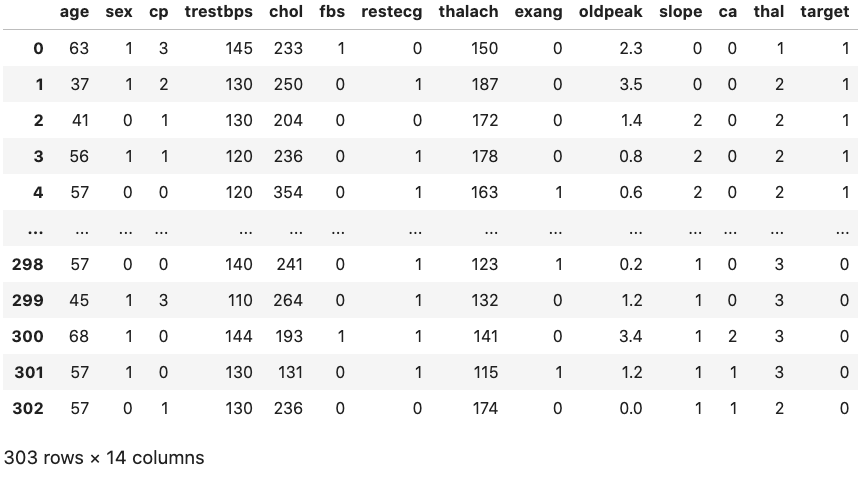 {width=70%}
\normalsize
\vspace{1.5ex}
\footnotesize
\textcolor{gray}{03_ml_basics_log_regr_heart_disease.ipynb}
\normalsize
{width=70%}
\normalsize
\vspace{1.5ex}
\footnotesize
\textcolor{gray}{03_ml_basics_log_regr_heart_disease.ipynb}
\normalsize
Example 2: Heart disease data set (logistic regression) (2)
\footnotesize
\textcolor{gray}{Define array of labels and feature vectors}
y = df['target'].values
X = df[[col for col in df.columns if col!="target"]]
\vfill \textcolor{gray}{Generate training and test data sets}
from sklearn.model_selection import train_test_split
X_train, X_test, y_train, y_test
		= train_test_split(X, y, test_size=0.5, shuffle=True)
\vfill \textcolor{gray}{Fit the model}
from sklearn.linear_model import LogisticRegression
lr = LogisticRegression(penalty='none',
		fit_intercept=True, max_iter=1000, tol=1E-5)
lr.fit(X_train, y_train)
\normalsize
Example 2: Heart disease data set (logistic regression) (3)
\footnotesize \textcolor{gray}{Test predictions on test data set:}
from sklearn.metrics import classification_report
y_pred_lr = lr.predict(X_test)
print(classification_report(y_test, y_pred_lr))
\vfill \textcolor{gray}{Output:}
              precision    recall  f1-score   support

           0       0.75      0.86      0.80        63
           1       0.89      0.80      0.84        89

    accuracy                           0.82       152
   macro avg       0.82      0.83      0.82       152
weighted avg       0.83      0.82      0.82       152
Example 2: Heart disease data set (logistic regression) (4)
\textcolor{gray}{Compare to another classifier using the \textit{receiver operating characteristic} (ROC) curve} \vfill \textcolor{gray}{Let's take the random forest classifier} \footnotesize
from sklearn.ensemble import RandomForestClassifier
rf = RandomForestClassifier(max_depth=3)
rf.fit(X_train, y_train)
\normalsize \vfill \textcolor{gray}{Use \texttt{roc_curve} from scikit-learn} \footnotesize
from sklearn.metrics import roc_curve

y_pred_prob_lr = lr.predict_proba(X_test) # predicted probabilities
fpr_lr, tpr_lr, _ = roc_curve(y_test, y_pred_prob_lr[:,1])

y_pred_prob_rf = rf.predict_proba(X_test) # predicted probabilities
fpr_rf, tpr_rf, _ = roc_curve(y_test, y_pred_prob_rf[:,1])
\normalsize
Example 2: Heart disease data set (logistic regression) (5)
::: columns :::: {.column width=50%} \scriptsize
plt.plot(tpr_lr, 1-fpr_lr, label="log. regression")
plt.plot(tpr_rf, 1-fpr_rf, label="random forest")
\vspace{5ex}
\normalsize \textcolor{gray}{Classifiers can be compared with the \textit{area under curve} (AUC) score.} \scriptsize
from sklearn.metrics import roc_auc_score
auc_lr = roc_auc_score(y_test,y_pred_lr)
auc_rf = roc_auc_score(y_test,y_pred_rf)
print(f"AUC scores: {auc_lr:.2f}, {auc_knn:.2f}")
\vspace{5ex} \normalsize \textcolor{gray}{This gives} \scriptsize
AUC scores: 0.82, 0.83
\normalsize
:::: :::: {.column width=50%} \begin{figure} \centering \includegraphics[width=0.96\textwidth]{figures/03_ml_basics_log_regr_heart_disease.pdf} \end{figure} :::: :::
Multinomial logistic regression: Softmax function
In the previous example we considered two classes (0, 1). For multi-class classification, the logistic function can generalized to the softmax function. \vfill Now consider $k$ classes and let $s_i$ be the score for class $i$: $\vec s = (s_1, ..., s_k)$ \vfill A probability for class $i$ can be predicted with the softmax function: $$ \sigma(\vec s)i = \frac{e^{s_i}}{\sum{j=1}^k e^{s_j}} \quad \text{ for } \quad i = 1, ... , k $$ The softmax functions is often used as the last activation function of a neural network in order to predict probabilities in a classification task. \vfill Multinomial logistic regression is also known as softmax regression.
Example 3: Iris data set (softmax regression) (1)
Iris flower data set
- Introduced 1936 in a paper by Ronald Fisher
- Task: classify flowers
- Three species: iris setosa, iris virginica and iris versicolor
- Four features: petal width and length, sepal width/length, in centimeters
::: columns :::: {.column width=40%} \begin{figure} \centering \includegraphics[width=0.95\textwidth]{figures/iris_dataset.png} \end{figure} :::: :::: {.column width=60%}
\vspace{2ex}
\footnotesize \textcolor{gray}{03_ml_basics_iris_softmax_regression.ipynb}
\vspace{19ex}
\scriptsize https://archive.ics.uci.edu/ml/datasets/Iris
https://en.wikipedia.org/wiki/Iris_flower_data_set \normalsize :::: :::
Example 3: Iris data set (softmax regression) (2)
\textcolor{gray}{Get data set} \footnotesize
# import some data to play with
# columns: Sepal Length, Sepal Width, Petal Length and Petal Width
iris = datasets.load_iris()
X = iris.data
y = iris.target

# split data into training and test data sets
x_train, x_test, y_train, y_test =
			train_test_split(X, y, test_size=0.5, random_state=42)
\normalsize \vfill
\textcolor{gray}{Softmax regression} \footnotesize
from sklearn.linear_model import LogisticRegression
log_reg = LogisticRegression(multi_class='multinomial', penalty='none')
log_reg.fit(x_train, y_train);
\normalsize
Example 3 : Iris data set (softmax regression) (3)
::: columns :::: {.column width=70%} \textcolor{gray}{Accuracy and confusion matrix for different classifiers} \footnotesize
for clf in [log_reg, kn_neigh, fisher_ld]:
    y_pred = clf.predict(x_test)
    acc = accuracy_score(y_test, y_pred)
    print(type(clf).__name__)
    print(f"accuracy: {acc:0.2f}")

    # confusion matrix:
    # columns: true class, row: predicted class
    print(confusion_matrix(y_test, y_pred),"\n")
\normalsize :::: :::: {.column width=30%}
\footnotesize
LogisticRegression
accuracy: 0.96
[[29  0  0]
 [ 0 23  0]
 [ 0  3 20]]

KNeighborsClassifier
accuracy: 0.95
[[29  0  0]
 [ 0 23  0]
 [ 0  4 19]]

LinearDiscriminantAnalysis
accuracy: 0.99
[[29  0  0]
 [ 0 23  0]
 [ 0  1 22]]
\normalsize :::: :::
General remarks on multi-variate analyses (MVAs)
- MVA Methods
- More effective than classic cut-based analyses
- Take correlations of input variables into account \vfill
- Important: find good input variables for MVA methods
- Good separation power between S and B
- No strong correlation among variables
- No correlation with the parameters you try to measure in your signal sample! \vfill
- Pre-processing
- Apply obvious variable transformations and let MVA method do the rest
- Make use of obvious symmetries: if e.g. a particle production process is symmetric in polar angle $\theta$ use $|\cos \theta|$ and not $\cos \theta$ as input variable
- It is generally useful to bring all input variables to a similar numerical range
Example of feature transformation
\begin{figure} \centering \includegraphics[width=0.95\textwidth]{figures/feature_transformation.png} \end{figure}
Exercise 1: Classification of air showers measured with the MAGIC telescope
::: columns :::: {.column width=50%}
\small
- Cosmic gamma rays (30 GeV - 30 TeV).
- Cherenkov light from air showers
- Background: air showers caused by hadrons. \normalsize
\begin{figure}
\centering
\includegraphics[width=0.85\textwidth]{figures/magic_photo_small.png}
\end{figure}
::::
:::: {.column width=50%}
 ::::
:::
::::
:::
Exercise 1: Classification of air showers measured with the MAGIC telescope
\begin{figure} \centering \includegraphics[width=0.75\textwidth]{figures/magic_shower_em_had_small.png} \end{figure} ::: columns :::: {.column width=50%} \begin{center} Gamma shower \end{center} :::: :::: {.column width=50%} \begin{center} Hadronic shower \end{center} :::: :::
Exercise 1: Classification of air showers measured with the MAGIC telescope
\begin{figure} \centering \includegraphics[width=0.95\textwidth]{figures/magic_shower_parameters.png} \end{figure}
Exercise 1: Classification of air showers measured with the MAGIC telescope
MAGIC data set
\tiny
\textcolor{gray}{https://archive.ics.uci.edu/ml/datasets/magic+gamma+telescope}
\normalsize
\scriptsize
1.  fLength:  continuous  # major axis of ellipse [mm]
2.  fWidth:   continuous  # minor axis of ellipse [mm]
3.  fSize:    continuous  # 10-log of sum of content of all pixels [in #phot]
4.  fConc:    continuous  # ratio of sum of two highest pixels over fSize  [ratio]
5.  fConc1:   continuous  # ratio of highest pixel over fSize  [ratio]
6.  fAsym:    continuous  # dist. from highest pixel to center, proj. onto major axis [mm]
7.  fM3Long:  continuous  # 3rd root of third moment along major axis  [mm]
8.  fM3Trans: continuous  # 3rd root of third moment along minor axis  [mm]
9.  fAlpha:   continuous  # angle of major axis with vector to origin [deg]
10. fDist:    continuous  # distance from origin to center of ellipse [mm]
11. class:    g,h         # gamma (signal), hadron (background)

g = gamma (signal):     12332
h = hadron (background): 6688

For technical reasons, the number of h events is underestimated.
In the real data, the h class represents the majority of the events.
\normalsize
Exercise 1: Classification of air showers measured with the MAGIC telescope
\small \textcolor{gray}{03_ml_basics_ex_1_magic.ipynb} \normalsize
a) Create for each variable a figure with a plot for gammas and hadrons overlayed. b) Create training and test data set. The test data should amount to 50% of the total data set. c) Define the logistic regressor and fit the training data d) Determine the model accuracy and the AUC score e) Plot the ROC curve (background rejection vs signal efficiency)
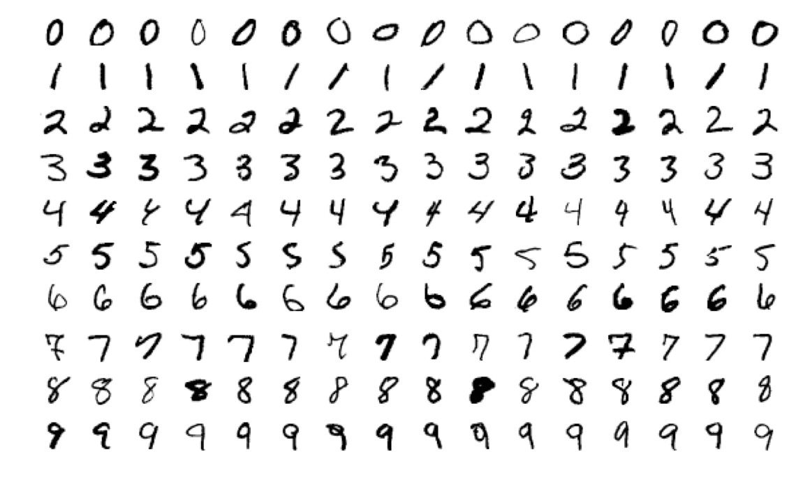
Exercise 2: Hand-written digit recognition with logistic regression
\small \textcolor{gray}{03_ml_basics_ex_2_mnist_softmax_regression.ipynb} \normalsize
a) Define logistic regressor from scikit-learn and fit data b) Use \texttt{classification_report} from scikit-learn to determine precision and recall c) Read in a hand-written digit and classify it. Print the probabilities for each digit. Determine the digit with the highest probability. d) (Optional) Create you own hand-written digit with a program like gimp and check what the classifier does
\begin{figure} \centering \includegraphics[width=0.85\textwidth]{figures/handwritten_digits.png} \end{figure}
Hint: You can install required packages on the jupyter hub server like so: \scriptsize
!pip3 install --user pypng
\normalsize
Exercise 3: Data preprocessing
a) Read the description of the sklearn.preprocessing package.
b) Start from the example notebook on the logistic regression for the heart disease data set (03_ml_basics_log_regr_heart_disease.ipynb). Pre-process the heart disease data set according to the given example. Does preprocessing make a difference in this case?