30 KiB
% Introduction to Data Analysis and Machine Learning in Physics: \ 1. Introduction to python % Day 1: 11. April 2023 % \underline{Jörg Marks}, Klaus Reygers
Outline of the $1^{st}$ day
-
Technical instructions for your interactions with the CIP pool, like
- using the jupyter hub
- using python locally in your own linux environment (anaconda)
- access the CIP pool from your own windows or linux system
- transfer data from and to the CIP pool
Can be found in \textcolor{violet}{CIPpoolAccess.PDF}\normalsize
-
Summary of NumPy
-
Plotting with matplotlib
-
Input / output of data
-
Summary of pandas
-
Fitting with iminuit and PyROOT
A glimpse into python classes
The following python classes are important to \textcolor{red}{data analysis and machine learning} and will be useful during the course
-
\textcolor{violet}{NumPy} - python library adding support for large, multi-dimensional arrays and matrices, along with high-level mathematical functions to operate on these arrays
-
\textcolor{violet}{matplotlib} - a python plotting library
-
\textcolor{violet}{SciPy} - extension of NumPy by a collection of mathematical algorithms for minimization, regression, fourier transformation, linear algebra and image processing
-
\textcolor{violet}{iminuit} - python wrapper to the data fitting toolkit \textcolor{violet}{Minuit2} developed at CERN by F. James in the 1970ies
-
\textcolor{violet}{PyROOT} - python wrapper to the C++ data analysis toolkit ROOT \textcolor{violet}{(lecture WS 2021 / 22)} used at the LHC
-
\textcolor{violet}{scikit-learn} - machine learning library written in python, which makes use extensively of NumPy for high-performance linear algebra algorithms
-
\textcolor{violet}{Tensorflow} - machine learning library with Keras as python interface
NumPy
\textcolor{blue}{NumPy} (Numerical Python) is an open source python library, which contains multidimensional array and matrix data structures and methods to efficiently operate on these. The core object is a homogeneous n-dimensional array object, \textcolor{blue}{ndarray}, which allows for a wide variety of \textcolor{blue}{fast operations and mathematical calculations with arrays and matrices} due to the extensive usage of compiled code.
-
It is heavily used in numerous scientific python packages
-
ndarray's have a fixed size at creation $\rightarrow$ changing size leads to recreation -
Array elements are all required to be of the same data type
-
Facilitates advanced mathematical operations on large datasets
-
See for a summary, e.g.
\small \textcolor{violet}{https://cs231n.github.io/python-numpy-tutorial/#numpy} \normalsize
\vfill
::: columns :::: {.column width=30%}
:::: :::
::: columns :::: {.column width=35%}
c = []
for i in range(len(a)):
c.append(a[i]*b[i])
::::
:::: {.column width=35%}
with NumPy
c = a * b
:::: :::
NumPy - array basics (1)
- numpy arrays build a grid of \textcolor{blue}{same type} values, which are indexed. The rank is the dimension of the array. There are methods to create and preset arrays.
\footnotesize
	 myA = np.array([12, 5 , 11])            # create rank 1 array (vector like)
	 type(myA)                               # <class ‘numpy.ndarray’>
	 myA.shape                               # (3,)
	 print(myA[2])                           # 11   access 3. element
	 myA[0] = 12                             # set 1. element to 12
	 myB = np.array([[1,5],[7,9]])           # create  rank 2 array
	 myB.shape                               # (2,2) (rows,columns)
	 print(myB[0,0],myB[0,1],myB[1,1])       # 1 5 9
	 myC = np.arange(6)                      # create rank 1 set to 0 - 5
	 myC.reshape(2,3)                        # change rank to (2,3)

	 zero = np.zeros((2,5))                  # 2 rows, 5 columns, set to 0
	 one = np.ones((2,2))                    # 2 rows, 2 columns, set to 1
	 five = np.full((2,2), 5)                # 2 rows, 2 columns, set to 5
	 e = np.eye(2)                           # create 2x2 identity matrix
\normalsize
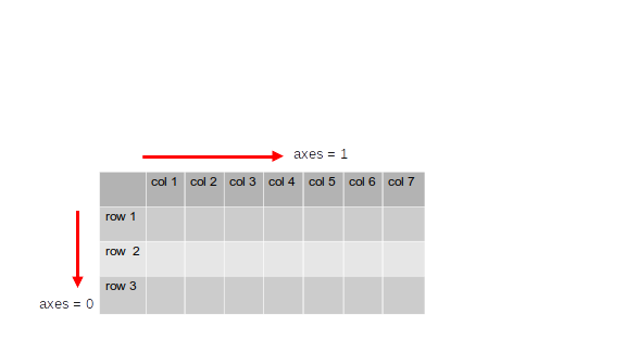
NumPy - array basics (2)
- Similar to a coordinate system numpy arrays also have \textcolor{blue}{axes}. numpy operations can be performed along these axes.
\footnotesize ::: columns :::: {.column width=35%}
# 2D arrays
five = np.full((2,3), 5)                # 2 rows, 3 columns, set to 5
seven = np.full((2,3), 7)               # 2 rows, 3 columns, set to 7
np.concatenate((five,seven), axis = 0)  # results in a 3 x 4 array
np.concatenate((five,seven), axis = 1]) # results in a 6 x 2 array
# 1D array
one = np.array([1, 1 , 1])              # results in a 1 x 3 array, set to 1
four = np.array([4, 4 , 4])             # results in a 1 x 3 array, set to 4
np.concatenate((one,four), axis = 0)    # concat. arrays horizontally!
::::
:::: {.column width=50%}
\vspace{3cm}
 ::::
:::
\normalsize
::::
:::
\normalsize
NumPy - array indexing (1)
- select slices of a numpy array
\footnotesize
     a = np.array([[1,2,3,4],
                   [5,6,7,8],                # 3 rows 4 columns array
                   [9,10,11,12]])
     b = a[:2, 1:3]                          # subarray of 2 rows and
         array([[2, 3],                      # column 1 and 2
                [6, 7]])
\normalsize
- a slice of an array points into the same data, modifying changes the original array!
\footnotesize
     b[0, 0] = 77	                         # b[0,0] and a[0,1] are 77

     r1_row = a[1, :]                        # get 2nd row ->  rank 1
     r1_row.shape	                         # (4,)
     r2_row = a[1:2, :]                      # get 2nd row -> rank 2
     r2_row.shape                            # (1,4)
     a=np.array([[1,2],[3,4],[5,6]])         # set a , 3 rows 2 cols
     d=a[[0, 1, 2], [0, 1, 1]]               # d contains [1 4 6]
     e=a[[1, 2], [1, 1]]                     # e contains [4 6]
     np.array([a[0,0],a[1,1],a[2,0]])        # address elements explicitly
\normalsize
NumPy - array indexing (2)
- integer array indexing by setting an array of indices $\rightarrow$ selecting/changing elements
\footnotesize
     a = np.array([[1,2,3,4],
                   [5,6,7,8],                # 3 rows 4 columns array
                   [9,10,11,12]])
     p_a = np.array([0,2,0])                 # Create an array of indices
     s = a[np.arange(3), p_a]                # number the rows, p_a points to cols
     print (s)                               # s contains [1 7 9]
     a[np.arange(3),p_a] += 10               # add 10 to corresponding elements
     x=np.array([[8,2],[7,4]])               # create 2x2 array
     bool = (x > 5)                          # bool : array of boolians
                                             #   [[True False]
                                             #    [True False]]
     print(x[x>5])                           # select elements, prints [8 7]
\normalsize
- data type in numpy - create according to input numbers or set explicitly
\footnotesize
     x = np.array([1.1, 2.1])                # create float array
     print(x.dtype)                          # print  float64
     y=np.array([1.1,2.9],dtype=np.int64)    # create float array [1 2]
\normalsize
NumPy - functions
- math functions operate elementwise either as operator overload or as methods
\footnotesize
     x=np.array([[1,2],[3,4]],dtype=np.float64)    # define 2x2 float array
     y=np.array([[3,1],[5,1]],dtype=np.float64)    # define 2x2 float array
     s = x + y                                     # elementwise sum
     s = np.add(x,y)
     s = np.subtract(x,y)
     s = np.multiply(x,y)                          # no matrix multiplication!
     s = np.divide(x,y)
     s = np.sqrt(x), np.exp(x), ...
     x @ y , or np.dot(x, y)                       # matrix product
     np.sum(x, axis=0)                             # sum of each column
     np.sum(x, axis=1)                             # sum of each row
     xT = x.T                                      # transpose of x
     x = np.linspace(0,2*pi,100)                   # get equal spaced points in x

     r = np.random.default_rng(seed=42)            # constructor random number class
     b = r.random((2,3))                           # random 2x3 matrix
\normalsize
-
broadcasting in numpy \vspace{0.4cm}
The term \textcolor{blue}{broadcasting} describes how numpy treats arrays with different shapes during arithmetic operations
-
add a scalar $b$ to a 1D array $a = [a_1,a_2,a_3]$ $\rightarrow$ expand $b$ to $[b,b,b]$ \vspace{0.2cm}
-
add a scalar $b$ to a 2D [2,3] array $a =a_{11},a_{12},a_{13}],[a_{21},a_{22},a_{23}$ $\rightarrow$ expand $b$ to $b =b,b,b],[b,b,b$ and add element wise \vspace{0.2cm}
-
add 1D array $b = [b_1,b_2,b_3]$ to a 2D [2,3] array $a=a_{11},a_{12},a_{13}],[a_{21},a_{22},a_{23}$ $\rightarrow$ 1D array is broadcast across each row of the 2D array $b =b_1,b_2,b_3],[b_1,b_2,b_3$ and added element wise \vspace{0.2cm}
Arithmetic operations can only be performed when the shape of each dimension in the arrays are equal or one has the dimension size of 1. Look \textcolor{violet}{here} for more details
-
\footnotesize
     # Add a vector to each row of a matrix
     x = np.array([[1,2,3], [4,5,6]]) # x has shape (2, 3)
     v = np.array([1,2,3])            # v has shape (3,)
     x + v     # [[2 4 6]
               #  [5 7 9]]
\normalsize
Plot data
A popular library to present data is the pyplot module of matplotlib.
- Drawing a function in one plot
\footnotesize ::: columns :::: {.column width=35%}
import numpy as np
import matplotlib.pyplot as plt
# generate 100 points from 0 to 2 pi
x = np.linspace( 0, 10*np.pi, 100 )
f = np.sin(x)**2
# plot function
plt.plot(x,f,'blueviolet',label='sine')
plt.xlabel('x [radian]')
plt.ylabel('f(x)')
plt.title('Plot sin^2')
plt.legend(loc='upper right')
plt.axis([0,30,-0.1,1.2]) # limit the plot range

# show the plot
plt.show()
::::
:::: {.column width=40%}
 ::::
:::
::::
:::
\normalsize
- Drawing a scatter plot of data
\footnotesize ::: columns :::: {.column width=35%}
...

# create x,y data points
num = 75
x = range(num)
y = range(num) +  np.random.randint(0,num/1.5,num)
z = - (range(num) +  np.random.randint(0,num/3,num)) + num
# create colored scatter plot, sample 1
plt.scatter(x, y, color = 'green',
                  label='Sample 1')
# create colored scatter plot, sample 2
plt.scatter(x, z, color = 'orange',
                  label='Sample 2')
plt.title('scatter plot')
plt.xlabel('x')
plt.ylabel('y')
# description and plot
plt.legend()
plt.show()
::::
:::: {.column width=35%}
\vspace{3cm}
 ::::
:::
\normalsize
::::
:::
\normalsize
- Drawing a histogram of data
\footnotesize ::: columns :::: {.column width=35%}
...

# create normalized gaussian Distribution
g = np.random.normal(size=10000)
# histogram the data
plt.hist(g,bins=40)
# plot rotated histogram
plt.hist(g,bins=40,orientation='horizontal')
# normalize area to 1
plt.hist(g,bins=40,density=True)
# change color
plt.hist(g,bins=40,density=True,
   edgecolor='lightgreen',color='orange')
plt.title('Gaussian Histogram')
plt.xlabel('bin')
plt.ylabel('entries')
# description and plot
plt.legend(['Normalized distribution'])
plt.show()
::::
:::: {.column width=35%}
\vspace{3.5cm}
 ::::
:::
\normalsize
::::
:::
\normalsize
- Drawing subplots in one canvas
\footnotesize ::: columns :::: {.column width=35%}
...
g = np.exp(-0.2*x)
# create figure
plt.figure(num=2,figsize=(10.0,7.5),dpi=150,facecolor='lightgrey')
plt.suptitle('1 x 2 Plot')
# create subplot and plot first one
plt.subplot(1,2,1)
# plot first one
plt.title('exp(x)')
plt.xlabel('x')
plt.ylabel('g(x)')
plt.plot(x,g,'blueviolet')
# create subplot and plot second one
plt.subplot(1,2,2)
plt.plot(x,f,'orange')
plt.plot(x,f*g,'red')
plt.legend(['sine^2','exp*sine'])
# show the plot
plt.show()
::::
:::: {.column width=40%}
\vspace{3cm}
 ::::
:::
\normalsize
::::
:::
\normalsize
Image data
The image class of the matplotlib library can be used to load the image
to numpy arrays and to render the image.
-
There are 3 common formats for the numpy array
-
(M, N) scalar data used for greyscale images
-
(M, N, 3) for RGB images (each pixel has an array with RGB color attached)
-
(M, N, 4) for RGBA images (each pixel has an array with RGB color and transparency attached)
The method
imreadloads the image into anndarray, which can be manipulated.The method
imshowrenders the image data -
\vspace {2cm}
- Drawing pixel data and images
\footnotesize ::: columns :::: {.column width=50%}
....
# create data array with pixel postion and RGB color code
width, height = 200, 200
data = np.zeros((height, width, 3), dtype=np.uint8)
# red patch in the center
data[75:125, 75:125] = [255, 0, 0]
x = np.random.randint(0,width-1,100)
y = np.random.randint(0,height-1,100)
data[x,y]= [0,255,0] # 100 random green pixel
plt.imshow(data)
plt.show()
....
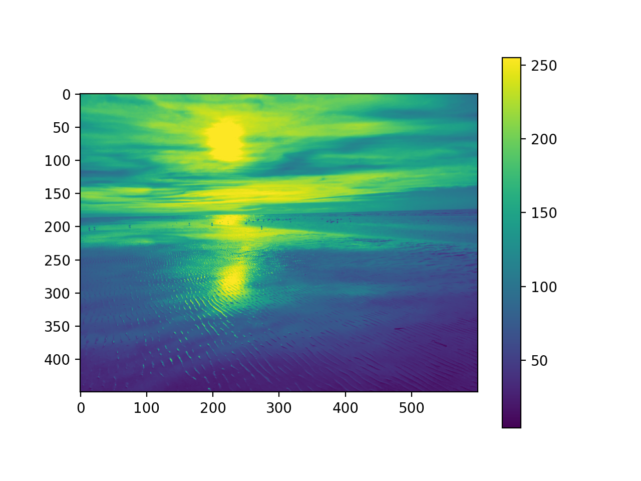
import matplotlib.image as mpimg
#read image into numpy array
pic = mpimg.imread('picture.jpg')
mod_pic = pic[:,:,0] # grab slice 0 of the colors
plt.imshow(mod_pic) # use default color code also
plt.colorbar() # try cmap='hot'
plt.show()
::::
:::: {.column width=25%}
 \vspace{1cm}
 ::::
:::
\normalsize
::::
:::
\normalsize
Input / output
For the analysis of measured data efficient input / output plays an
important role. In numpy, ndarrays can be saved and read in from files.
load() and save() functions handle numpy binary files (.npy extension)
which contain data, shape, dtype and other information required to
reconstruct the ndarray of the disk file.
\footnotesize
   r = np.random.default_rng()       # instanciate random number generator
   a = r.random((4,3))               # random 4x3 array
   np.save('myBinary.npy', a)        # write array a to binary file myBinary.npy
   b = np.arange(12)
   np.savez('myComp.npz', a=a, b=b)  # write a and b in compressed binary file
   ......
   b = np.load('myBinary.npy')       # read content of myBinary.npy into b
\normalsize
The storage and retrieval of array data in text file format is done
with savetxt() and loadtxt() methods. Parameter controlling delimiter,
line separators, file header and footer can be specified.
\footnotesize
   x = np.array([1,2,3,4,5,6,7])                      # create ndarray
   np.savetxt('myText.txt',x,fmt='%d', delimiter=',') # write array x to file myText.txt
                                                      # with comma separation
\normalsize
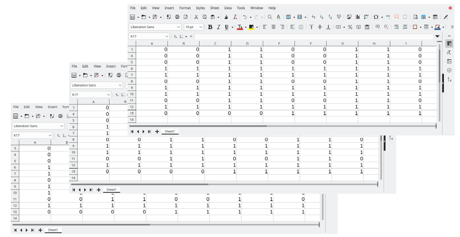
Input / output
Import tabular data from table processing programs in office packages.
\vspace{0.4cm}
\footnotesize
::: columns
:::: {.column width=35%}
Excel data can be exported as text file (myData_01.csv) with a comma as
delimiter.
::::
:::: {.column width=35%}
 ::::
:::
::::
:::
\footnotesize
   .....
   # read content of all files myData_*.csv into data
   data = np.loadtxt('myData_01.csv',dtype=int,delimiter=',')

   print (data.shape)               #  (12, 9)
   print (data)                     #  [[1 1 1 1 0 0 0 0 0]
                                    #   [0 0 1 1 0 0 1 1 0]
                                    #  .....
                                    #   [0 0 0 0 1 1 1 1 1]]
\normalsize
Input / output
Import tabular data from table processing programs in office packages.
\vspace{0.4cm}
\footnotesize
::: columns
:::: {.column width=35%}
Excel data can be exported as text file (myData_01.csv) with a comma as
delimiter. \newline
$\color{blue}{Often~many~files~are~available~(myData_*.csv)}$
::::
:::: {.column width=35%}
 ::::
:::
::::
:::
\footnotesize
   .....
   # find files and directories with names matching a pattern
   import glob
   # read content of all files myData_*.csv into data
   file_list = sorted(glob.glob('myData_*.csv')) # generate a sorted file list
   for filename in file_list:
       data = np.loadtxt(fname=filename, dtype=int, delimiter=',')
       print(data[:,3])     # print column 3 of each file
                            # [1 1 1 1 1 1 1 1 1 1 1 0]
                            # ......
                            # [0 1 0 1 0 1 0 1 0 1 0 1]
\normalsize
Exercise 1
i) Display a numpy array as figure of a blue cross. The size should be 200 by 200 pixel. Use as array format (M, N, 3), where the first 2 specify the pixel positions and the last 3 the rbg color from 0:255.
- Draw in addition a red square of arbitrary position into the figure.
- Draw a circle in the center of the figure. Try to create a mask which selects the inner part of the circle using the indexing.
\small Solution: 01_intro_ex_1a_sol.ipynb \normalsize
ii) Read data which contains pixels from the binary file horse.py into a numpy array. Display the data and the following transformations in 4 subplots: scaling and translation, compression in x and y, rotation and mirroring.
\small
[Solution: 01_intro_ex_1b_sol.ipynb](https://www.physi.uni-heidelberg.de/~reygers/lectures/2023/ml/solutions/01_intro_ex_1b_sol.ipynb) \normalsize
Pandas
\textcolor{violet}{pandas} is a software library written in python for \textcolor{blue}{data manipulation and analysis}.
\vspace{0.4cm}
\setbeamertemplate{itemize item}{\color{red}\tiny$\blacksquare$}
-
Offers data structures and operations for manipulating numerical tables with integrated indexing
-
Imports data from various file formats, e.g. comma-separated values, JSON, SQL or Excel
-
Tools for reading and writing data structures, allows analyzing, filtering, spliting, grouping and aggregating, merging and joining and plotting
-
Built on top of
NumPy -
Visualize the data with
matplotlib -
Most machine learning tools support
pandas$\rightarrow$ it is widely used to preprocess data sets for analysis and machine learning in various scientific fields
Pandas micro introduction
Goal: Exploring, cleaning, transforming, and visualization of data. The basic indexable objects are
\setbeamertemplate{itemize item}{\color{red}\tiny$\blacksquare$}
-
Series-> vector (list) of data elements of arbitrary type -
DataFrame-> tabular arangement of data elements of column wise arbitrary typeBoth allow cleaning data by removing of
emptyornandata entries
\footnotesize
     import numpy as np
     import pandas as pd                    # use together with numpy
     s = pd.Series([1, 3, 5, np.nan, 6, 8]) # create a Series of int64
     r = pd.Series(np.random.randn(4))      # Series of random numbers float64
     dates = pd.date_range("20130101", periods=3) # index according to dates
     df = pd.DataFrame(np.random.randn(3,4),index=dates,columns=list("ABCD"))
     print (df)                             # print the DataFrame
                        A         B         C         D
          2013-01-01  1.618395  1.210263 -1.276586 -0.775545
          2013-01-02  0.676783 -0.754161 -1.148029 -0.244821
          2013-01-03 -0.359081  0.296019  1.541571  0.235337

     new_s = s.dropna() # return a new Data Frame without the column that has NaN cells
\normalsize
\setbeamertemplate{itemize item}{\color{red}\tiny$\blacksquare$}
-
pandas data can be saved in different file formats (CSV, JASON, html, XML, Excel, OpenDocument, HDF5 format, .....).
NaNentries are kept in the output file, except if they are removed withdataframe.dropna()-
csv file \footnotesize
df.to_csv("myFile.csv") # Write the DataFrame df to a csv file\normalsize
-
HDF5 output
\footnotesize
df.to_hdf("myFile.h5",key='df',mode='w') # Write the DataFrame df to HDF5
s.to_hdf("myFile.h5", key='s',mode='a')
\normalsize
-
Writing to an excel file
\footnotesize
df.to_excel("myFile.xlsx", sheet_name="Sheet1")\normalsize
-
-
Deleting file with data in python
\footnotesize
     import os
     os.remove('myFile.h5')
\normalsize
\setbeamertemplate{itemize item}{\color{red}\tiny$\blacksquare$}
-
read in data from various formats
-
csv file
\footnotesize
 .......
 df = pd.read_csv('heart.csv')  # read csv data table
 print(df.info())
    <class 'pandas.core.frame.DataFrame'>
    RangeIndex: 303 entries, 0 to 302
    Data columns (total 14 columns):
    #   Column    Non-Null Count  Dtype
    ---  ------    --------------  -----
    0   age       303 non-null    int64
    1   sex       303 non-null    int64
    2   cp        303 non-null    int64
    print(df.head(5))       # prints the first 5 rows of the data table
    print(df.describe())    # shows a quick statistic summary of your data
-
\normalsize
-
Reading an excel file
\footnotesize
df = pd.read_excel("myFile.xlsx","Sheet1", na_values=["NA"])\normalsize
\textcolor{olive}{There are many options specifying details for IO.}
\setbeamertemplate{itemize item}{\color{red}\tiny$\blacksquare$}
-
Various functions exist to select and view data from pandas objects
-
Display column and index
\footnotesize
df.index                    # show datetime index of df
DatetimeIndex(['2013-01-01','2013-01-02','2013-01-03'],
              dtype='datetime64[ns]',freq='D')
df.column                   # show columns info
Index(['A', 'B', 'C', 'D'], dtype='object')
\normalsize
-
DataFrame.to_numpy()gives aNumPyrepresentation of the underlying data\footnotesize
df.to_numpy()       # one dtype for the entire array, not per column!
[[-0.62660101 -0.67330526  0.23269168 -0.67403546]
[-0.53033339  0.32872063 -0.09893568  0.44814084]
[-0.60289996 -0.22352548 -0.43393248  0.47531456]]
\normalsize
Does not include the index or column labels in the output
-
more on viewing
\footnotesize
df.T                                   # transpose the DataFrame df
df.sort_values(by="B")                 # Sorting by values of column B of df
df.sort_index(axis=0)                  # Sorting by index ascending values
df.sort_index(axis=0,ascending=False)  # Display columns in inverse order
\normalsize
-
\setbeamertemplate{itemize item}{\color{red}\tiny$\blacksquare$}
-
Selecting data of pandas objects $\rightarrow$ keep or reduce dimensions
-
get a named column as a Series
\footnotesize
df["A"]           # selects a column A from df, simular to  df.A
df.iloc[:, 1:2]   # slices column A explicitly from df, df.loc[:, ["A"]]
\normalsize
-
select rows of a DataFrame
\footnotesize
df[0:2]                   # selects row 0 and 1 from df,
df["20130102":"20130103"] # use indices, endpoints are included!
df.iloc[3]                # select with the position of the passed integers
df.iloc[1:3, :]           # selects row 1 and 2 from df
\normalsize
-
select by label
\footnotesize
df.loc["20130102":"20130103",["C","D"]] # selects row 1 and 2 and only C and D
df.loc[dates[0], "A"]                   # selects a single value (scalar)
\normalsize
-
select by lists of integer position (as in
NumPy)\footnotesize
df.iloc[[0, 2], [1, 3]] # select row 1 and 3 and col B and D (data only)
df.iloc[1, 1]           # get a value explicitly (data only, no index lines)
\normalsize
-
select according to expressions
\footnotesize
df.query('B<C')         # select rows where B < C
df1=df[(df["B"]==0)&(df["D"]==0)] # conditions on rows
\normalsize
-
\setbeamertemplate{itemize item}{\color{red}\tiny$\blacksquare$}
-
Selecting data of pandas objects continued
-
Boolean indexing
\footnotesize
df[df["A"] > 0]           # select df where all values of column A are >0
df[df > 0]                # select values >0 from the entire DataFrame
\normalsize
more complex example
\footnotesize
df2 = df.copy()                     # copy df
df2["E"] = ["eight","one","four"]   # add column E
df2[df2["E"].isin(["two", "four"])] # test if elements "two" and  "four" are
                                    # contained in Series column E
\normalsize
-
Operations (in general exclude missing data)
\footnotesize
df2[df2 > 0] = -df2   # All elements > 0 change sign
df.mean(0)            # get column wise mean (numbers=axis)
df.mean(1)            # get row wise mean
df.std(0)             # standard deviation according to axis
df.cumsum()           # cumulative sum of each column
df.apply(np.sin)      # apply function to each element of df
df.apply(lambda x: x.max() - x.min()) # apply lambda function column wise
df + 10               # add scalar 10
df - [1, 2, 10 , 100] # subtract values of each column
df.corr()             # Compute pairwise correlation of columns
\normalsize
-
\setbeamertemplate{itemize item}{\color{red}\tiny$\blacksquare$}
-
Selecting data of pandas objects continued
\vspace{0.5cm}
-
More operations
\footnotesize
df.drop(['col1', 'col2'], axis=1)  # removes columns 'col1' and 'col2'
df.fillna(0)                       # fills missing values with 0
df.fillna(method='ffill')          # fills missing values with previous
                                   # non-missing value in the column
df.replace('old_val', 'new_val')   # replaces 'old_val' with 'new_val'
df.groupby('col1').mean()          # groups by 'col1' and computes
                                   # the mean of each group
pd.merge(df1, df2, on='column1')   # merges df1 and df2 on 'column1'
df['column1'].value_counts()       # counts the number of occurrences
                                   # of each unique value in 'column'
\normalsize
\vspace{3cm}
-
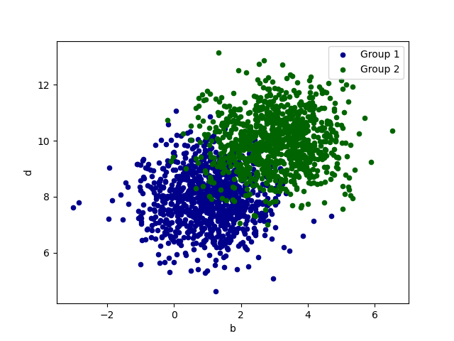
Pandas - plotting data
\textcolor{violet}{Visualization} is integrated in pandas using matplotlib. Here are only 2 examples
- Plot random data in histogramm and scatter plot
\footnotesize
     # create DataFrame with random normal distributed data
     df = pd.DataFrame(np.random.randn(1000,4),columns=["a","b","c","d"])
     df = df + [1, 3, 8 , 10]      # shift column wise mean by  1, 3, 8 , 10
     df.plot.hist(bins=20)         # histogram all 4 columns
     g1 = df.plot.scatter(x="a",y="c",color="DarkBlue",label="Group 1")
     df.plot.scatter(x="b",y="d",color="DarkGreen",label="Group 2",ax=g1)
\normalsize
::: columns
:::: {.column width=35%}
 ::::
:::: {.column width=35%}
::::
:::: {.column width=35%}
 ::::
:::
::::
:::
Pandas - plotting data
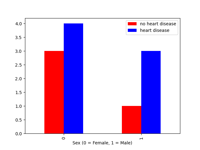
The function crosstab() takes one or more array-like objects as indexes or columns and constructs a new DataFrame of variable counts on the inputs
\footnotesize
   df = pd.DataFrame(                # create DataFrame of 2 categories
      {"sex":   np.array([0,0,0,0,1,1,1,1,0,0,0]),
       "heart": np.array([1,1,1,0,1,1,1,0,0,0,1])
      }  )                           # closing bracket goes on next line
   pd.crosstab(df2.sex,df2.heart)    # create cross table of possibilities
   pd.crosstab(df2.sex,df2.heart).plot(kind="bar",color=['red','blue']) # plot counts
\normalsize
::: columns
:::: {.column width=38%}
 ::::
:::
::::
:::
Exercise 2
Read the file \textcolor{violet}{heart.csv} into a DataFrame. \textcolor{violet}{Information on the dataset}
\setbeamertemplate{itemize item}{\color{red}$\square$}
-
Which columns do we have
-
Print the first 3 rows
-
Print the statistics summary and the correlations
-
Print mean values for each column with and without disease (target)
-
Select the data according to
sexandtarget(heart disease 0=no 1=yes). -
Plot the
agedistribution of male and female in one histogram -
Plot the heart disease distribution according to chest pain type
cp -
Plot
thalachaccording totargetin one histogramm -
Plot
sexandtargetin a histogramm figure -
Correlate
ageandmax heart rateaccording totarget -
Correlate
ageandcolesterolaccording totarget
\small Solution: 01_intro_ex_2_sol.ipynb \normalsize